# GetDist Documentation
---
## https://getdist.readthedocs.io/en/latest/index.html
# GetDist
GetDist is a Python package for analysing and plotting Monte Carlo (or other) samples.
* [Introduction](intro.md)
* [Plot gallery and tutorial](https://getdist.readthedocs.io/en/latest/plot_gallery.html)
* [GetDist GUI program](gui.md)
* [Paper with technical details](https://arxiv.org/abs/1910.13970)
**LLM Integration**: For AI assistants and LLM agents, a comprehensive [LLM context document](https://getdist.readthedocs.io/en/latest/_static/getdist_docs_combined.md) can be used.
There’s also an [AI help assistant](https://cosmocoffee.info/help_assist.php) you can use to ask about the package.
High-level modules for analysing samples and plotting:
* [getdist.mcsamples](mcsamples.md)
* [`loadMCSamples()`](mcsamples.md#getdist.mcsamples.loadMCSamples)
* [`MCSamples`](mcsamples.md#getdist.mcsamples.MCSamples)
* [getdist.plots](plots.md)
* [getdist.plots.get_single_plotter](_summaries/getdist.plots.get_single_plotter.md)
* [getdist.plots.get_subplot_plotter](_summaries/getdist.plots.get_subplot_plotter.md)
* [getdist.plots.GetDistPlotter](_summaries/getdist.plots.GetDistPlotter.md)
* [getdist.plots.GetDistPlotSettings](_summaries/getdist.plots.GetDistPlotSettings.md)
* [`GetDistPlotError`](plots.md#getdist.plots.GetDistPlotError)
* [`GetDistPlotSettings`](plots.md#getdist.plots.GetDistPlotSettings)
* [`GetDistPlotter`](plots.md#getdist.plots.GetDistPlotter)
* [`MCSampleAnalysis`](plots.md#getdist.plots.MCSampleAnalysis)
* [`add_plotter_style()`](plots.md#getdist.plots.add_plotter_style)
* [`get_plotter()`](plots.md#getdist.plots.get_plotter)
* [`get_single_plotter()`](plots.md#getdist.plots.get_single_plotter)
* [`get_subplot_plotter()`](plots.md#getdist.plots.get_subplot_plotter)
* [`set_active_style()`](plots.md#getdist.plots.set_active_style)
See also:
* [Analysis settings](analysis_settings.md)
* [Using GetDist with MCMC sampler outputs](arviz_integration.md)
* [ArviZ Integration](arviz_integration.md#arviz-integration)
* [Basic Usage](arviz_integration.md#basic-usage)
* [PyMC Integration](arviz_integration.md#pymc-integration)
* [Example: Eight Schools Model](arviz_integration.md#example-eight-schools-model)
* [emcee Integration](arviz_integration.md#emcee-integration)
* [ArviZ Options](arviz_integration.md#arviz-options)
* [Custom Parameter Ranges](arviz_integration.md#custom-parameter-ranges)
* [Including Weights and Likelihoods](arviz_integration.md#including-weights-and-likelihoods)
* [Multi-dimensional Parameters](arviz_integration.md#multi-dimensional-parameters)
* [Burn in](arviz_integration.md#burn-in)
Other main modules:
* [getdist.chains](chains.md)
* [getdist.covmat](covmat.md)
* [getdist.densities](densities.md)
* [getdist.gaussian_mixtures](gaussian_mixtures.md)
* [getdist.inifile](inifile.md)
* [getdist.paramnames](paramnames.md)
* [getdist.parampriors](parampriors.md)
* [getdist.types](types.md)
* [Index](genindex.md)
---
[](https://www.sussex.ac.uk/astronomy/)[](https://erc.europa.eu/)[](https://stfc.ukri.org/)
## https://getdist.readthedocs.io/en/latest/mcsamples.html
# getdist.mcsamples
#### NOTE
**Important Convention**: In GetDist, the `loglikes` parameter and related variables represent
**-log(posterior)**, not -log(likelihood). The posterior is the product of likelihood and prior.
This means `loglikes` contains the negative logarithm of the full
posterior probability, including both the likelihood and any prior contributions.
### getdist.mcsamples.loadMCSamples(file_root: [str](https://docs.python.org/3/library/stdtypes.html#str), ini: [None](https://docs.python.org/3/library/constants.html#None) | [str](https://docs.python.org/3/library/stdtypes.html#str) | [IniFile](inifile.md#getdist.inifile.IniFile) = None, jobItem=None, no_cache=False, settings: [Mapping](https://docs.python.org/3/library/collections.abc.html#collections.abc.Mapping)[[str](https://docs.python.org/3/library/stdtypes.html#str), [Any](https://docs.python.org/3/library/typing.html#typing.Any)] | [None](https://docs.python.org/3/library/constants.html#None) = None, chain_exclude=None) → [MCSamples](#getdist.mcsamples.MCSamples)
Loads a set of samples from a file or files.
Sample files are plain text (*file_root.txt*) or a set of files (*file_root_1.txt*, *file_root_2.txt*, etc.).
Auxiliary files **file_root.paramnames** gives the parameter names
and (optionally) **file_root.ranges** gives hard prior parameter ranges.
For a description of the various analysis settings and default values see
[analysis_defaults.ini](https://getdist.readthedocs.io/en/latest/analysis_settings.html).
* **Parameters:**
* **file_root** – The root name of the files to read (no extension)
* **ini** – The name of a .ini file with analysis settings to use
* **jobItem** – an optional grid jobItem instance for a CosmoMC grid output
* **no_cache** – Indicates whether or not we should cache loaded samples in a pickle
* **settings** – dictionary of analysis settings to override defaults
* **chain_exclude** – A list of indexes to exclude, None to include all
* **Returns:**
The [`MCSamples`](#getdist.mcsamples.MCSamples) instance
### *class* getdist.mcsamples.MCSamples(root: [str](https://docs.python.org/3/library/stdtypes.html#str) | [None](https://docs.python.org/3/library/constants.html#None) = None, jobItem=None, ini=None, settings: [Mapping](https://docs.python.org/3/library/collections.abc.html#collections.abc.Mapping)[[str](https://docs.python.org/3/library/stdtypes.html#str), [Any](https://docs.python.org/3/library/typing.html#typing.Any)] | [None](https://docs.python.org/3/library/constants.html#None) = None, ranges=None, samples: [ndarray](https://numpy.org/doc/stable/reference/generated/numpy.ndarray.html#numpy.ndarray) | [Iterable](https://docs.python.org/3/library/collections.abc.html#collections.abc.Iterable)[[ndarray](https://numpy.org/doc/stable/reference/generated/numpy.ndarray.html#numpy.ndarray)] | [None](https://docs.python.org/3/library/constants.html#None) = None, weights: [ndarray](https://numpy.org/doc/stable/reference/generated/numpy.ndarray.html#numpy.ndarray) | [Iterable](https://docs.python.org/3/library/collections.abc.html#collections.abc.Iterable)[[ndarray](https://numpy.org/doc/stable/reference/generated/numpy.ndarray.html#numpy.ndarray)] | [None](https://docs.python.org/3/library/constants.html#None) = None, loglikes: [ndarray](https://numpy.org/doc/stable/reference/generated/numpy.ndarray.html#numpy.ndarray) | [Iterable](https://docs.python.org/3/library/collections.abc.html#collections.abc.Iterable)[[ndarray](https://numpy.org/doc/stable/reference/generated/numpy.ndarray.html#numpy.ndarray)] | [None](https://docs.python.org/3/library/constants.html#None) = None, temperature: [float](https://docs.python.org/3/library/functions.html#float) | [None](https://docs.python.org/3/library/constants.html#None) = None, \*\*kwargs)
The main high-level class for a collection of parameter samples.
Derives from [`chains.Chains`](chains.md#getdist.chains.Chains), adding high-level functions including
Kernel Density estimates, parameter ranges and custom settings.
For a description of the various analysis settings and default values see
[analysis_defaults.ini](https://getdist.readthedocs.io/en/latest/analysis_settings.html).
* **Parameters:**
* **root** – A root file name when loading from file
* **jobItem** – optional jobItem for parameter grid item. Should have jobItem.chainRoot and jobItem.batchPath
* **ini** – a .ini file to use for custom analysis settings
* **settings** – a dictionary of custom analysis settings
* **ranges** – a dictionary giving any additional hard prior bounds for parameters, or if periodic,
e.g. {‘x’:[0, 1], ‘y’:[None,2]}
If a parameter is periodic, use a triplet, e.g. {‘phi’: [0, 2\*np.pi, True]}
* **samples** – if not loading from file, array of parameter values for each sample, passed
to [`setSamples()`](#getdist.mcsamples.MCSamples.setSamples), or list of arrays if more than one chain
* **weights** – array of weights for samples, or list of arrays if more than one chain
* **loglikes** – array of -log(posterior) for samples, or list of arrays if more than one chain.
Note: this is the negative log posterior (likelihood × prior), not just the likelihood.
* **temperatute** – temperature of the sample. If not specified will be read from the
root.properties.ini file if it exists and otherwise default to 1.
* **kwargs** –
keyword arguments passed to inherited classes, e.g. to manually make a samples object from
: sample arrays in memory:
- **paramNamesFile**: optional name of .paramnames file with parameter names
- **names**: list of names for the parameters, or list of arrays if more than one chain
- **labels**: list of latex labels for the parameters (without $…$)
- **renames**: dictionary of parameter aliases
- **ignore_rows**:
> - if int >=1: The number of rows to skip at the file in the beginning of the file
> - if float <1: The fraction of rows to skip at the beginning of the file
- **label**: a latex label for the samples
- **name_tag**: a name tag for this instance
- **sampler**: string describing the type of samples; if “nested” or “uncorrelated”
the effective number of samples is calculated using uncorrelated approximation. If not specified
will be read from the root.properties.ini file if it exists and otherwise default to “mcmc”.
#### PCA(params, param_map=None, normparam=None, writeDataToFile=False, filename=None, conditional_params=(), n_best_only=None)
Perform principal component analysis (PCA). In other words,
get eigenvectors and eigenvalues for normalized variables
with optional (log modulus) mapping to find power law fits.
* **Parameters:**
* **params** – List of names of the parameters to use
* **param_map** – A transformation to apply to parameter values; A list or string containing
either N (no transformation) or L (for log transform) for each parameter.
By default, uses log if no parameter values cross zero
* **normparam** – optional name of parameter to normalize result (i.e. this parameter will have unit power)
* **writeDataToFile** – True to write the output to file.
* **filename** – The filename to write, by default root_name.PCA.
* **conditional_params** – optional list of parameters to treat as fixed,
i.e. for PCA conditional on fixed values of these parameters
* **n_best_only** – return just the short summary constraint for the tightest n_best_only constraints
* **Returns:**
a string description of the output of the PCA
#### addDerived(paramVec, name, label='', comment='', range=None)
Adds a new derived parameter
* **Parameters:**
* **paramVec** – The vector of parameter values to add. For example a combination of
parameter arrays from MCSamples.getParams()
* **name** – The name for the new parameter
* **label** – optional latex label for the parameter
* **comment** – optional comment describing the parameter
* **range** – if specified, a tuple of min, max values for the new parameter hard prior bounds
(either can be None for one-side bound)
* **Returns:**
The added parameter’s [`ParamInfo`](paramnames.md#getdist.paramnames.ParamInfo) object
#### changeSamples(samples)
Sets the samples without changing weights and loglikes.
* **Parameters:**
**samples** – The samples to set
#### confidence(paramVec, limfrac, upper=False, start=0, end=None, weights=None) → [ndarray](https://numpy.org/doc/stable/reference/generated/numpy.ndarray.html#numpy.ndarray)
Calculate sample confidence limits, not using kernel densities just counting samples in the tails
* **Parameters:**
* **paramVec** – array of parameter values or int index of parameter to use
* **limfrac** – fraction of samples in the tail,
e.g. 0.05 for a 95% one-tail limit, or 0.025 for a 95% two-tail limit
* **upper** – True to get upper limit, False for lower limit
* **start** – Start index for the vector to use
* **end** – The end index, use None to go all the way to the end of the vector.
* **weights** – numpy array of weights for each sample, by default self.weights
* **Returns:**
confidence limit (parameter value when limfac of samples are further in the tail)
#### cool(cool=None)
Cools the samples, i.e. multiplies log likelihoods by cool factor and re-weights accordingly
:param cool: cool factor, optional if the sample has a temperature specified.
#### copy(label=None, settings=None) → [MCSamples](#getdist.mcsamples.MCSamples)
Create a copy of this sample object
* **Parameters:**
* **label** – optional lable for the new copy
* **settings** – optional modified settings for the new copy
* **Returns:**
copyied [`MCSamples`](#getdist.mcsamples.MCSamples) instance
#### corr(pars=None)
Get the correlation matrix
* **Parameters:**
**pars** – If specified, list of parameter vectors or int indices to use
* **Returns:**
The correlation matrix.
#### cov(pars=None, where=None)
Get parameter covariance
* **Parameters:**
* **pars** – if specified, a list of parameter vectors or int indices to use
* **where** – if specified, a filter for the samples to use
(where x>=5 would mean only process samples with x>=5).
* **Returns:**
The covariance matrix
#### deleteFixedParams()
Delete parameters that are fixed (the same value in all samples).
This includes parameters that are all NaN.
#### deleteZeros()
Removes samples with zero weight
#### filter(where)
Filter the stored samples to keep only samples matching filter
* **Parameters:**
**where** – list of sample indices to keep, or boolean array filter (e.g. x>5 to keep only samples where x>5)
#### get1DDensity(name, \*\*kwargs)
Returns a [`Density1D`](densities.md#getdist.densities.Density1D) instance for parameter with given name. Result is cached.
* **Parameters:**
* **name** – name of the parameter
* **kwargs** – arguments for [`get1DDensityGridData()`](#getdist.mcsamples.MCSamples.get1DDensityGridData)
* **Returns:**
A [`Density1D`](densities.md#getdist.densities.Density1D) instance for parameter with given name
#### get1DDensityGridData(j, paramConfid=None, meanlikes=False, \*\*kwargs)
Low-level function to get a [`Density1D`](densities.md#getdist.densities.Density1D) instance for the marginalized 1D density
of a parameter. Result is not cached.
* **Parameters:**
* **j** – a name or index of the parameter
* **paramConfid** – optional cached [`ParamConfidenceData`](chains.md#getdist.chains.ParamConfidenceData) instance
* **meanlikes** – include mean likelihoods
* **kwargs** –
optional settings to override instance settings of the same name (see analysis_settings):
- **smooth_scale_1D**
- **boundary_correction_order**
- **mult_bias_correction_order**
- **fine_bins**
- **num_bins**
* **Returns:**
A [`Density1D`](densities.md#getdist.densities.Density1D) instance
#### get2DDensity(x, y, normalized=False, \*\*kwargs)
Returns a [`Density2D`](densities.md#getdist.densities.Density2D) instance with marginalized 2D density.
* **Parameters:**
* **x** – index or name of x parameter
* **y** – index or name of y parameter
* **normalized** – if False, is normalized so the maximum is 1, if True, density is normalized
* **kwargs** – keyword arguments for the [`get2DDensityGridData()`](#getdist.mcsamples.MCSamples.get2DDensityGridData) function
* **Returns:**
[`Density2D`](densities.md#getdist.densities.Density2D) instance
#### get2DDensityGridData(j, j2, num_plot_contours=None, get_density=False, meanlikes=False, mask_function: callable = None, \*\*kwargs)
Low-level function to get 2D plot marginalized density and optional additional plot data.
* **Parameters:**
* **j** – name or index of the x parameter
* **j2** – name or index of the y parameter.
* **num_plot_contours** – number of contours to calculate and return in density.contours
* **get_density** – only get the 2D marginalized density, don’t calculate confidence level members
* **meanlikes** – calculate mean likelihoods as well as marginalized density
(returned as array in density.likes)
* **mask_function** – optional function, mask_function(minx, miny, stepx, stepy, mask),
which which sets mask to zero for values of parameters that are excluded by prior. Note this is not
needed for standard min, max bounds aligned with axes, as they are handled by default.
* **kwargs** –
optional settings to override instance settings of the same name (see analysis_settings):
- **fine_bins_2D**
- **boundary_correction_order**
- **mult_bias_correction_order**
- **smooth_scale_2D**
* **Returns:**
a [`Density2D`](densities.md#getdist.densities.Density2D) instance
#### getAutoBandwidth1D(bins, par, param, mult_bias_correction_order=None, kernel_order=1, N_eff=None)
Get optimized kernel density bandwidth (in units of the range of the bins)
Based on optimal Improved Sheather-Jones bandwidth for basic Parzen kernel, then scaled if higher-order method
being used. For details see the notes at [arXiv:1910.13970](https://arxiv.org/abs/1910.13970).
* **Parameters:**
* **bins** – numpy array of binned weights for the samples
* **par** – A [`ParamInfo`](paramnames.md#getdist.paramnames.ParamInfo) instance for the parameter to analyse
* **param** – index of the parameter to use
* **mult_bias_correction_order** – order of multiplicative bias correction (0 is basic Parzen kernel);
by default taken from instance settings.
* **kernel_order** – order of the kernel
(0 is Parzen, 1 does linear boundary correction, 2 is a higher-order kernel)
* **N_eff** – effective number of samples. If not specified estimated using weights, autocorrelations,
and fiducial bandwidth
* **Returns:**
kernel density bandwidth (in units the range of the bins)
#### getAutoBandwidth2D(bins, parx, pary, paramx, paramy, corr, rangex, rangey, base_fine_bins_2D, mult_bias_correction_order=None, min_corr=0.2, N_eff=None, use_2D_Neff=False)
Get optimized kernel density bandwidth matrix in parameter units, using Improved Sheather Jones method in
sheared parameters. The shearing is determined using the covariance, so you know the distribution is
multi-modal, potentially giving ‘fake’ correlation, turn off shearing by setting min_corr=1.
For details see the notes [arXiv:1910.13970](https://arxiv.org/abs/1910.13970).
* **Parameters:**
* **bins** – 2D numpy array of binned weights
* **parx** – A [`ParamInfo`](paramnames.md#getdist.paramnames.ParamInfo) instance for the x parameter
* **pary** – A [`ParamInfo`](paramnames.md#getdist.paramnames.ParamInfo) instance for the y parameter
* **paramx** – index of the x parameter
* **paramy** – index of the y parameter
* **corr** – correlation of the samples
* **rangex** – scale in the x parameter
* **rangey** – scale in the y parameter
* **base_fine_bins_2D** – number of bins to use for re-binning in rotated parameter space
* **mult_bias_correction_order** – multiplicative bias correction order (0 is Parzen kernel); by default taken
from instance settings
* **min_corr** – minimum correlation value at which to bother de-correlating the parameters
* **N_eff** – effective number of samples. If not specified, uses rough estimate that accounts for
weights and strongly-correlated nearby samples (see notes)
* **use_2D_Neff** – if N_eff not specified, whether to use 2D estimate of effective number, or approximate from
the 1D results (default from use_effective_samples_2D setting)
* **Returns:**
kernel density bandwidth matrix in parameter units
#### getAutocorrelation(paramVec, maxOff=None, weight_units=True, normalized=True)
Gets auto-correlation of an array of parameter values (e.g. for correlated samples from MCMC)
By default, uses weight units (i.e. standard units for separate samples from original chain).
If samples are made from multiple chains, neglects edge effects.
* **Parameters:**
* **paramVec** – an array of parameter values, or the int index of the parameter in stored samples to use
* **maxOff** – maximum autocorrelation distance to return
* **weight_units** – False to get result in sample point (row) units; weight_units=False gives standard
definition for raw chains
* **normalized** – Set to False to get covariance
(note even if normalized, corr[0]<>1 in general unless weights are unity).
* **Returns:**
zero-based array giving auto-correlations
#### getBestFit(max_posterior=True)
> Returns a [`BestFit`](types.md#getdist.types.BestFit) object with best-fit point stored in .minimum or .bestfit file
* **Parameters:**
**max_posterior** – whether to get maximum posterior (from .minimum file)
or maximum likelihood (from .bestfit file)
* **Returns:**
#### getBounds()
Returns the bounds in the form of a [`ParamBounds`](parampriors.md#getdist.parampriors.ParamBounds) instance, for example
for determining plot ranges
Bounds are not the same as self.ranges, as if samples are not near the range boundary, the bound is set to None
* **Returns:**
a [`ParamBounds`](parampriors.md#getdist.parampriors.ParamBounds) instance
#### getCombinedSamplesWithSamples(samps2, sample_weights=(1, 1))
Make a new [`MCSamples`](#getdist.mcsamples.MCSamples) instance by appending samples from samps2 for parameters which are in common.
By defaultm they are weighted so that the probability mass of each set of samples is the same,
independent of tha actual sample sizes. The sample_weights parameter can be adjusted to change the
relative weighting.
* **Parameters:**
* **samps2** – [`MCSamples`](#getdist.mcsamples.MCSamples) instance to merge
* **sample_weights** – relative weights for combining the samples. Set to None to just directly append samples.
* **Returns:**
a new [`MCSamples`](#getdist.mcsamples.MCSamples) instance with the combined samples
#### getConvergeTests(test_confidence=0.95, writeDataToFile=False, what=('MeanVar', 'GelmanRubin', 'SplitTest', 'RafteryLewis', 'CorrLengths'), filename=None, feedback=False)
Do convergence tests.
* **Parameters:**
* **test_confidence** – confidence limit to test for convergence (two-tail, only applies to some tests)
* **writeDataToFile** – True to write output to a file
* **what** –
The tests to run. Should be a list of any of the following:
- ’MeanVar’: Gelman-Rubin sqrt(var(chain mean)/mean(chain var)) test in individual parameters (multiple chains only)
- ’GelmanRubin’: Gelman-Rubin test for the worst orthogonalized parameter (multiple chains only)
- ’SplitTest’: Crude test for variation in confidence limits when samples are split up into subsets
- ’RafteryLewis’: [Raftery-Lewis test](https://stat.uw.edu/sites/default/files/files/reports/1991/tr212.pdf) (integer weight samples only)
- ’CorrLengths’: Sample correlation lengths
* **filename** – The filename to write to, default is file_root.converge
* **feedback** – If set to True, Prints the output as well as returning it.
* **Returns:**
text giving the output of the tests
#### getCorrelatedVariable2DPlots(num_plots=12, nparam=None)
Gets a list of most correlated variable pair names.
* **Parameters:**
* **num_plots** – The number of plots
* **nparam** – maximum number of pairs to get
* **Returns:**
list of [x,y] pair names
#### getCorrelationLength(j, weight_units=True, min_corr=0.05, corr=None)
Gets the auto-correlation length for parameter j
* **Parameters:**
* **j** – The index of the parameter to use
* **weight_units** – False to get result in sample point (row) units; weight_units=False gives standard
definition for raw chains
* **min_corr** – specifies a minimum value of the autocorrelation to use, e.g. where sampling noise is
typically as large as the calculation
* **corr** – The auto-correlation array to use, calculated internally by default
using [`getAutocorrelation()`](#getdist.mcsamples.MCSamples.getAutocorrelation)
* **Returns:**
the auto-correlation length
#### getCorrelationMatrix()
Get the correlation matrix of all parameters
* **Returns:**
The correlation matrix
#### getCov(nparam=None, pars=None)
Get covariance matrix of the parameters. By default, uses all parameters, or can limit to max number or list.
* **Parameters:**
* **nparam** – if specified, only use the first nparam parameters
* **pars** – if specified, a list of parameter indices (0,1,2..) to include
* **Returns:**
covariance matrix.
#### getCovMat()
Gets the CovMat instance containing covariance matrix for all the non-derived parameters
(for example useful for subsequent MCMC runs to orthogonalize the parameters)
* **Returns:**
A [`CovMat`](covmat.md#getdist.covmat.CovMat) object holding the covariance
#### getEffectiveSamples(j=0, min_corr=0.05)
Gets effective number of samples N_eff so that the error on mean of parameter j is sigma_j/N_eff
* **Parameters:**
* **j** – The index of the param to use.
* **min_corr** – the minimum value of the auto-correlation to use when estimating the correlation length
#### getEffectiveSamplesGaussianKDE(paramVec, h=0.2, scale=None, maxoff=None, min_corr=0.05)
Roughly estimate an effective sample number for use in the leading term for the MISE
(mean integrated squared error) of a Gaussian-kernel KDE (Kernel Density Estimate). This is used for
optimizing the kernel bandwidth, and though approximate should be better than entirely ignoring sample
correlations, or only counting distinct samples.
Uses fiducial assumed kernel scale h; result does depend on this (typically by factors O(2))
For bias-corrected KDE only need very rough estimate to use in rule of thumb for bandwidth.
In the limit h-> 0 (but still >0) answer should be correct (then just includes MCMC rejection duplicates).
In reality correct result for practical h should depend on shape of the correlation function.
If self.sampler is ‘nested’ or ‘uncorrelated’ return result for uncorrelated samples.
* **Parameters:**
* **paramVec** – parameter array, or int index of parameter to use
* **h** – fiducial assumed kernel scale.
* **scale** – a scale parameter to determine fiducial kernel width, by default the parameter standard deviation
* **maxoff** – maximum value of auto-correlation length to use
* **min_corr** – ignore correlations smaller than this auto-correlation
* **Returns:**
A very rough effective sample number for leading term for the MISE of a Gaussian KDE.
#### getEffectiveSamplesGaussianKDE_2d(i, j, h=0.3, maxoff=None, min_corr=0.05)
Roughly estimate an effective sample number for use in the leading term for the 2D MISE.
If self.sampler is ‘nested’ or ‘uncorrelated’ return result for uncorrelated samples.
* **Parameters:**
* **i** – parameter array, or int index of first parameter to use
* **j** – parameter array, or int index of second parameter to use
* **h** – fiducial assumed kernel scale.
* **maxoff** – maximum value of auto-correlation length to use
* **min_corr** – ignore correlations smaller than this auto-correlation
* **Returns:**
A very rough effective sample number for leading term for the MISE of a Gaussian KDE.
#### getFractionIndices(weights, n)
Calculates the indices of weights that split the weights into sets of equal 1/n fraction of the total weight
* **Parameters:**
* **weights** – array of weights
* **n** – number of groups to split into
* **Returns:**
array of indices of the boundary rows in the weights array
#### getGelmanRubin(nparam=None, chainlist=None)
Assess the convergence using the maximum var(mean)/mean(var) of orthogonalized parameters
c.f. Brooks and Gelman 1997.
* **Parameters:**
* **nparam** – The number of parameters, by default uses all
* **chainlist** – list of [`WeightedSamples`](chains.md#getdist.chains.WeightedSamples), the samples to use. Defaults to all the
separate chains in this instance.
* **Returns:**
The worst var(mean)/mean(var) for orthogonalized parameters. Should be <<1 for good convergence.
#### getGelmanRubinEigenvalues(nparam=None, chainlist=None)
Assess convergence using var(mean)/mean(var) in the orthogonalized parameters
c.f. Brooks and Gelman 1997.
* **Parameters:**
* **nparam** – The number of parameters (starting at first), by default uses all of them
* **chainlist** – list of [`WeightedSamples`](chains.md#getdist.chains.WeightedSamples), the samples to use.
Defaults to all the separate chains in this instance.
* **Returns:**
array of var(mean)/mean(var) for orthogonalized parameters
#### getInlineLatex(param, limit=1, err_sig_figs=None)
Get snippet like: A=x\\pm y. Will adjust appropriately for one and two tail limits.
* **Parameters:**
* **param** – The name of the parameter
* **limit** – which limit to get, 1 is the first (default 68%), 2 is the second
(limits array specified by self.contours)
* **err_sig_figs** – significant figures in the error
* **Returns:**
The tex snippet.
#### getLabel()
Return the latex label for the samples
* **Returns:**
the label
#### getLatex(params=None, limit=1, err_sig_figs=None)
Get tex snippet for constraints on a list of parameters
* **Parameters:**
* **params** – list of parameter names, or a single parameter name
* **limit** – which limit to get, 1 is the first (default 68%), 2 is the second
(limits array specified by self.contours)
* **err_sig_figs** – significant figures in the error
* **Returns:**
labels, texs: a list of parameter labels, and a list of tex snippets,
or for a single parameter, the latex snippet.
#### getLikeStats()
Get best fit sample and n-D confidence limits, and various likelihood based statistics
* **Returns:**
a [`LikeStats`](types.md#getdist.types.LikeStats) instance storing N-D limits for parameter i in
result.names[i].ND_limit_top, result.names[i].ND_limit_bot, and best-fit sample value
in result.names[i].bestfit_sample
#### getLower(name)
Return the lower limit of the parameter with the given name.
* **Parameters:**
**name** – parameter name
* **Returns:**
The lower limit if name exists, None otherwise.
#### getMargeStats(include_bestfit=False)
Returns a [`MargeStats`](types.md#getdist.types.MargeStats) object with marginalized 1D parameter constraints
* **Parameters:**
**include_bestfit** – if True, set best fit values by loading from root_name.minimum file (assuming it exists)
* **Returns:**
A [`MargeStats`](types.md#getdist.types.MargeStats) instance
#### getMeans(pars=None)
Gets the parameter means, from saved array if previously calculated.
* **Parameters:**
**pars** – optional list of parameter indices to return means for
* **Returns:**
numpy array of parameter means
#### getName()
Returns the name tag of these samples.
* **Returns:**
The name tag
#### getNumSampleSummaryText()
Returns a summary text describing numbers of parameters and samples,
and various measures of the effective numbers of samples.
* **Returns:**
The summary text as a string.
#### getParamBestFitDict(best_sample=False, want_derived=True, want_fixed=True, max_posterior=True)
Gets a dictionary of parameter values for the best fit point,
assuming calculated results from mimimization runs in .minimum (max posterior) .bestfit (max likelihood)
files exists.
Can also get the best-fit (max posterior) sample, which typically has a likelihood that differs significantly
from the true best fit in high dimensions.
* **Parameters:**
* **best_sample** – load from global minimum files (False, default) or using maximum posterior sample (True)
* **want_derived** – include derived parameters
* **want_fixed** – also include values of any fixed parameters
* **max_posterior** – whether to get maximum posterior (from .minimum file) or maximum likelihood
(from .bestfit file)
* **Returns:**
dictionary of parameter values
#### getParamNames()
Get [`ParamNames`](paramnames.md#getdist.paramnames.ParamNames) object with names for the parameters
* **Returns:**
[`ParamNames`](paramnames.md#getdist.paramnames.ParamNames) object giving parameter names and labels
#### getParamSampleDict(ix, want_derived=True, want_fixed=True)
Gets a dictionary of parameter values for sample number ix
* **Parameters:**
* **ix** – index of the sample to return (zero based)
* **want_derived** – include derived parameters
* **want_fixed** – also include values of any fixed parameters
* **Returns:**
dictionary of parameter values
#### getParams()
Creates a [`ParSamples`](chains.md#getdist.chains.ParSamples) object, with variables giving vectors for all the parameters,
for example samples.getParams().name1 would be the vector of samples with name ‘name1’
* **Returns:**
A [`ParSamples`](chains.md#getdist.chains.ParSamples) object containing all the parameter vectors, with attributes
given by the parameter names
#### getRawNDDensity(xs, normalized=False, \*\*kwargs)
Returns a `DensityND` instance with marginalized ND density.
* **Parameters:**
* **xs** – indices or names of x_i parameters
* **kwargs** – keyword arguments for the `getNDDensityGridData()` function
* **normalized** – if False, is normalized so the maximum is 1, if True, density is normalized
* **Returns:**
[`DensityND`](densities.md#getdist.densities.DensityND) instance
#### getRawNDDensityGridData(js, writeDataToFile=False, num_plot_contours=None, get_density=False, meanlikes=False, maxlikes=False, \*\*kwargs)
Low-level function to get unsmooth ND plot marginalized
density and optional additional plot data.
* **Parameters:**
* **js** – vector of names or indices of the x_i parameters
* **writeDataToFile** – save outputs to file
* **num_plot_contours** – number of contours to calculate and return in density.contours
* **get_density** – only get the ND marginalized density, no additional plot data, no contours.
* **meanlikes** – calculate mean likelihoods as well as marginalized density
(returned as array in density.likes)
* **maxlikes** – calculate the profile likelihoods in addition to the others
(returned as array in density.maxlikes)
* **kwargs** – optional settings to override instance settings of the same name (see analysis_settings):
* **Returns:**
a [`DensityND`](densities.md#getdist.densities.DensityND) instance
#### getRenames()
Gets dictionary of renames known to each parameter.
#### getSeparateChains() → [list](https://docs.python.org/3/library/stdtypes.html#list)[[WeightedSamples](chains.md#getdist.chains.WeightedSamples)]
Gets a list of samples for separate chains.
If the chains have already been combined, uses the stored sample offsets to reconstruct the array
(generally no array copying)
* **Returns:**
The list of [`WeightedSamples`](chains.md#getdist.chains.WeightedSamples) for each chain.
#### getSignalToNoise(params, noise=None, R=None, eigs_only=False)
Returns w, M, where w is the eigenvalues of the signal to noise (small y better constrained)
* **Parameters:**
* **params** – list of parameters indices to use
* **noise** – noise matrix
* **R** – rotation matrix, defaults to inverse of Cholesky root of the noise matrix
* **eigs_only** – only return eigenvalues
* **Returns:**
w, M, where w is the eigenvalues of the signal to noise (small y better constrained)
#### getTable(columns=1, include_bestfit=False, \*\*kwargs)
Creates and returns a [`ResultTable`](types.md#getdist.types.ResultTable) instance. See also [`getInlineLatex()`](#getdist.mcsamples.MCSamples.getInlineLatex).
* **Parameters:**
* **columns** – number of columns in the table
* **include_bestfit** – True to include the bestfit parameter values (assuming set)
* **kwargs** – arguments for [`ResultTable`](types.md#getdist.types.ResultTable) constructor.
* **Returns:**
A [`ResultTable`](types.md#getdist.types.ResultTable) instance
#### getUpper(name)
Return the upper limit of the parameter with the given name.
* **Parameters:**
**name** – parameter name
* **Returns:**
The upper limit if name exists, None otherwise.
#### getVars()
Get the parameter variances
* **Returns:**
A numpy array of variances.
#### get_norm(where=None)
gets the normalization, the sum of the sample weights: sum_i w_i
* **Parameters:**
**where** – if specified, a filter for the samples to use
(where x>=5 would mean only process samples with x>=5).
* **Returns:**
normalization
#### initParamConfidenceData(paramVec, start=0, end=None, weights=None)
Initialize cache of data for calculating confidence intervals
* **Parameters:**
* **paramVec** – array of parameter values or int index of parameter to use
* **start** – The sample start index to use
* **end** – The sample end index to use, use None to go all the way to the end of the vector
* **weights** – A numpy array of weights for each sample, defaults to self.weights
* **Returns:**
[`ParamConfidenceData`](chains.md#getdist.chains.ParamConfidenceData) instance
#### initParameters(ini)
Initializes settings.
Gets parameters from [`IniFile`](inifile.md#getdist.inifile.IniFile).
* **Parameters:**
**ini** – The [`IniFile`](inifile.md#getdist.inifile.IniFile) to be used
#### loadChains(root, files_or_samples: [Sequence](https://docs.python.org/3/library/collections.abc.html#collections.abc.Sequence), weights=None, loglikes=None, ignore_lines=None)
Loads chains from files.
* **Parameters:**
* **root** – Root name
* **files_or_samples** – list of file names or list of arrays of samples, or single array of samples
* **weights** – if loading from arrays of samples, corresponding list of arrays of weights
* **loglikes** – if loading from arrays of samples, corresponding list of arrays of -log(posterior)
* **ignore_lines** – Amount of lines at the start of the file to ignore, None not to ignore any
* **Returns:**
True if loaded successfully, False if none loaded
#### makeSingle()
Combines separate chains into one samples array, so self.samples has all the samples
and this instance can then be used as a general [`WeightedSamples`](chains.md#getdist.chains.WeightedSamples) instance.
* **Returns:**
self
#### makeSingleSamples(filename='', single_thin=None, random_state=None)
Make file of unit weight samples by choosing samples
with probability proportional to their weight.
If you just want the indices of the samples use
[`random_single_samples_indices()`](chains.md#getdist.chains.WeightedSamples.random_single_samples_indices) instead.
* **Parameters:**
* **filename** – The filename to write to, leave empty if no output file is needed
* **single_thin** – factor to thin by; if not set generates as many samples as it can
up to self.max_scatter_points
* **random_state** – random seed or Generator
* **Returns:**
numpy array of selected weight-1 samples if no filename
#### mean(paramVec, where=None)
Get the mean of the given parameter vector.
* **Parameters:**
* **paramVec** – array of parameter values or int index of parameter to use
* **where** – if specified, a filter for the samples to use
(where x>=5 would mean only process samples with x>=5).
* **Returns:**
parameter mean
#### mean_diff(paramVec, where=None)
Calculates an array of differences between a parameter vector and the mean parameter value
* **Parameters:**
* **paramVec** – array of parameter values or int index of parameter to use
* **where** – if specified, a filter for the samples to use
(where x>=5 would mean only process samples with x>=5).
* **Returns:**
array of p_i - mean(p_i)
#### mean_diffs(pars: [None](https://docs.python.org/3/library/constants.html#None) | [int](https://docs.python.org/3/library/functions.html#int) | [Sequence](https://docs.python.org/3/library/collections.abc.html#collections.abc.Sequence) = None, where=None) → [Sequence](https://docs.python.org/3/library/collections.abc.html#collections.abc.Sequence)
Calculates a list of parameter vectors giving distances from parameter means
* **Parameters:**
* **pars** – if specified, list of parameter vectors or int parameter indices to use
* **where** – if specified, a filter for the samples to use
(where x>=5 would mean only process samples with x>=5).
* **Returns:**
list of arrays p_i-mean(p-i) for each parameter
#### parLabel(i)
Gets the latex label of the parameter
* **Parameters:**
**i** – The index or name of a parameter.
* **Returns:**
The parameter’s label.
#### parName(i, starDerived=False)
Gets the name of i’th parameter
* **Parameters:**
* **i** – The index of the parameter
* **starDerived** – add a star at the end of the name if the parameter is derived
* **Returns:**
The name of the parameter (string)
#### random_single_samples_indices(random_state=None, thin: [float](https://docs.python.org/3/library/functions.html#float) | [None](https://docs.python.org/3/library/constants.html#None) = None, max_samples: [int](https://docs.python.org/3/library/functions.html#int) | [None](https://docs.python.org/3/library/constants.html#None) = None)
Returns an array of sample indices that give a list of weight-one samples, by randomly
selecting samples depending on the sample weights
* **Parameters:**
* **random_state** – random seed or Generator
* **thin** – additional thinning factor (>1 to get fewer samples)
* **max_samples** – optional parameter to thin to get a specified mean maximum number of samples
* **Returns:**
array of sample indices
#### readChains(files_or_samples, weights=None, loglikes=None)
Loads samples from a list of files or array(s), removing burn in,
deleting fixed parameters, and combining into one self.samples array
* **Parameters:**
* **files_or_samples** – The list of file names to read, samples or list of samples
* **weights** – array of weights if setting from arrays
* **loglikes** – array of -log(posterior) if setting from arrays
* **Returns:**
self.
#### removeBurn(remove=0.3)
removes burn in from the start of the samples
* **Parameters:**
**remove** – fraction of samples to remove, or if int >1, the number of sample rows to remove
#### removeBurnFraction(ignore_frac)
Remove a fraction of the samples as burn in
* **Parameters:**
**ignore_frac** – fraction of sample points to remove from the start of the samples, or each chain
if not combined
#### reweightAddingLogLikes(logLikes)
Importance sample the samples, by adding logLike (array of -log(likelihood values)) to the currently
stored likelihoods, and re-weighting accordingly, e.g. for adding a new data constraint.
* **Parameters:**
**logLikes** – array of -log(likelihood) for each sample to adjust
#### saveAsText(root, chain_index=None, make_dirs=False)
Saves the samples as text files, including parameter names as .paramnames file.
* **Parameters:**
* **root** – The root name to use
* **chain_index** – Optional index to be used for the filename, zero based, e.g. for saving one
of multiple chains
* **make_dirs** – True if this should (recursively) create the directory if it doesn’t exist
#### savePickle(filename)
Save the current object to a file in pickle format
* **Parameters:**
**filename** – The file to write to
#### saveTextMetadata(root, properties=None)
Saves metadata about the sames to text files with given file root
* **Parameters:**
* **root** – root file name
* **properties** – optional dictiory of values to save in root.properties.ini
#### setColData(coldata, are_chains=True)
Set the samples given an array loaded from file
* **Parameters:**
* **coldata** – The array with columns of [weights, -log(Likelihoods)] and sample parameter values
* **are_chains** – True if coldata starts with two columns giving weight and -log(Likelihood)
#### setDiffs()
saves self.diffs array of parameter differences from the y, e.g. to later calculate variances etc.
* **Returns:**
array of differences
#### setMeans()
Calculates and saves the means of the samples
* **Returns:**
numpy array of parameter means
#### setMinWeightRatio(min_weight_ratio=1e-30)
Removes samples with weight less than min_weight_ratio times the maximum weight
* **Parameters:**
**min_weight_ratio** – minimum ratio to max to exclude
#### setParamNames(names=None)
Sets the names of the params.
* **Parameters:**
**names** – Either a [`ParamNames`](paramnames.md#getdist.paramnames.ParamNames) object, the name of a .paramnames file to load, a list
of name strings, otherwise use default names (param1, param2…).
#### setParams(obj)
Adds array variables obj.name1, obj.name2 etc., where
obj.name1 is the vector of samples with name ‘name1’
if a parameter name is of the form aa.bb.cc, it makes subobjects so that you can reference obj.aa.bb.cc.
If aa.bb and aa are both parameter names, then aa becomes obj.aa.value.
* **Parameters:**
**obj** – The object instance to add the parameter vectors variables
* **Returns:**
The obj after alterations.
#### setRanges(ranges)
Sets the ranges parameters, e.g. hard priors on positivity etc.
If a min or max value is None, then it is assumed to be unbounded.
* **Parameters:**
**ranges** – A list or a tuple of [min,max] values for each parameter,
or a dictionary giving [min,max] values for specific parameter names.
For periodic parameters use dictionary with [min, max, True] entry.
#### setSamples(samples, weights=None, loglikes=None, min_weight_ratio=None)
Sets the samples from numpy arrays
* **Parameters:**
* **samples** – The sample values, n_samples x n_parameters numpy array, or can be a list of parameter vectors
* **weights** – Array of weights for each sample. Defaults to 1 for all samples if unspecified.
* **loglikes** – Array of -log(posterior) values for each sample.
* **min_weight_ratio** – remove samples with weight less than min_weight_ratio of the maximum
#### std(paramVec, where=None)
Get the standard deviation of the given parameter vector.
* **Parameters:**
* **paramVec** – array of parameter values or int index of parameter to use
* **where** – if specified, a filter for the samples to use
(where x>=5 would mean only process samples with x>=5).
* **Returns:**
parameter standard deviation.
#### thin(factor: [int](https://docs.python.org/3/library/functions.html#int))
Thin the samples by the given factor, giving set of samples with unit weight
* **Parameters:**
**factor** – The factor to thin by
#### thin_indices(factor, weights=None)
Indices to make single weight 1 samples. Assumes integer weights.
* **Parameters:**
* **factor** – The factor to thin by, should be int.
* **weights** – The weights to thin, None if this should use the weights stored in the object.
* **Returns:**
array of indices of samples to keep
#### *static* thin_indices_and_weights(factor, weights)
Returns indices and new weights for use when thinning samples.
* **Parameters:**
* **factor** – thin factor
* **weights** – initial weight (counts) per sample point
* **Returns:**
(unique index, counts) tuple of sample index values to keep and new weights
#### twoTailLimits(paramVec, confidence)
Calculates two-tail equal-area confidence limit by counting samples in the tails
* **Parameters:**
* **paramVec** – array of parameter values or int index of parameter to use
* **confidence** – confidence limit to calculate, e.g. 0.95 for 95% confidence
* **Returns:**
min, max values for the confidence interval
#### updateBaseStatistics()
Updates basic computed statistics (y, covariance etc.), e.g. after a change in samples or weights
* **Returns:**
self
#### updateRenames(renames)
Updates the renames known to each parameter with the given dictionary of renames.
#### updateSettings(settings: [Mapping](https://docs.python.org/3/library/collections.abc.html#collections.abc.Mapping)[[str](https://docs.python.org/3/library/stdtypes.html#str), [Any](https://docs.python.org/3/library/typing.html#typing.Any)] | [None](https://docs.python.org/3/library/constants.html#None) = None, ini: [None](https://docs.python.org/3/library/constants.html#None) | [str](https://docs.python.org/3/library/stdtypes.html#str) | [IniFile](inifile.md#getdist.inifile.IniFile) = None, doUpdate=True)
Updates settings from a .ini file or dictionary
* **Parameters:**
* **settings** – A dict containing settings to set, taking preference over any values in ini
* **ini** – The name of .ini file to get settings from, or an [`IniFile`](inifile.md#getdist.inifile.IniFile) instance; by default
uses current settings
* **doUpdate** – True if we should update internal computed values, False otherwise (e.g. if you want to make
other changes first)
#### var(paramVec, where=None)
Get the variance of the given parameter vector.
* **Parameters:**
* **paramVec** – array of parameter values or int index of parameter to use
* **where** – if specified, a filter for the samples to use
(where x>=5 would mean only process samples with x>=5).
* **Returns:**
parameter variance
#### weighted_sum(paramVec, where=None)
Calculates the weighted sum of a parameter vector, sum_i w_i p_i
* **Parameters:**
* **paramVec** – array of parameter values or int index of parameter to use
* **where** – if specified, a filter for the samples to use
(where x>=5 would mean only process samples with x>=5).
* **Returns:**
weighted sum
#### weighted_thin(factor: [int](https://docs.python.org/3/library/functions.html#int))
Thin the samples by the given factor, giving (in general) non-unit integer weights.
This function also preserves separate chains.
* **Parameters:**
**factor** – The (integer) factor to thin by
#### writeCorrelationMatrix(filename=None)
Write the correlation matrix to a file
* **Parameters:**
**filename** – The file to write to, If none writes to file_root.corr
#### writeCovMatrix(filename=None)
Writes the covrariance matrix of non-derived parameters to a file.
* **Parameters:**
**filename** – The filename to write to; default is file_root.covmat
#### writeThinData(fname, thin_ix, cool=1)
Writes samples at thin_ix to file
* **Parameters:**
* **fname** – The filename to write to.
* **thin_ix** – Indices of the samples to write
* **cool** – if not 1, cools the samples by this factor
### *exception* getdist.mcsamples.MCSamplesError
An Exception that is raised when there is an error inside the MCSamples class.
### *exception* getdist.mcsamples.ParamError
An Exception that indicates a bad parameter.
### *exception* getdist.mcsamples.SettingError
An Exception that indicates bad settings.
## https://getdist.readthedocs.io/en/latest/plots.html
# getdist.plots
This module is used for making plots from samples. The [`get_single_plotter()`](#getdist.plots.get_single_plotter) and [`get_subplot_plotter()`](#getdist.plots.get_subplot_plotter) functions are used to make a plotter instance,
which is then used to make and export plots.
Many plotter functions take a **roots** argument, which is either a root name for
some chain files, or an in-memory [`MCSamples`](mcsamples.md#getdist.mcsamples.MCSamples) instance. You can also make comparison plots by giving a list of either of these.
Parameter are referenced simply by name (as specified in the .paramnames file when loading from file, or set in the [`MCSamples`](mcsamples.md#getdist.mcsamples.MCSamples) instance).
For functions that takes lists of parameters, these can be just lists of names.
You can also use glob patterns to match specific subsets of parameters (e.g. *x\** to match all parameters with names starting with *x*).
| [`get_single_plotter`](#getdist.plots.get_single_plotter) | Get a [`GetDistPlotter`](#getdist.plots.GetDistPlotter) for making a single plot of fixed width. |
|-------------------------------------------------------------|----------------------------------------------------------------------------------------------------|
| [`get_subplot_plotter`](#getdist.plots.get_subplot_plotter) | Get a [`GetDistPlotter`](#getdist.plots.GetDistPlotter) for making an array of subplots. |
| [`GetDistPlotter`](#getdist.plots.GetDistPlotter) | Main class for making plots from one or more sets of samples. |
| [`GetDistPlotSettings`](#getdist.plots.GetDistPlotSettings) | Settings class (colors, sizes, font, styles etc.) |
### *exception* getdist.plots.GetDistPlotError
An exception that is raised when there is an error plotting
### *class* getdist.plots.GetDistPlotSettings(subplot_size_inch: [float](https://docs.python.org/3/library/functions.html#float) = 2, fig_width_inch: [float](https://docs.python.org/3/library/functions.html#float) | [None](https://docs.python.org/3/library/constants.html#None) = None)
Settings class (colors, sizes, font, styles etc.)
* **Variables:**
* **alpha_factor_contour_lines** – alpha factor for adding contour lines between filled contours
* **alpha_filled_add** – alpha for adding filled contours to a plot
* **axes_fontsize** – Size for axis font at reference axis size
* **axes_labelsize** – Size for axis label font at reference axis size
* **axis_marker_color** – The color for a marker
* **axis_marker_ls** – The line style for a marker
* **axis_marker_lw** – The line width for a marker
* **axis_tick_powerlimits** – exponents at which to use scientific notation for axis tick labels
* **axis_tick_max_labels** – maximum number of tick labels per axis
* **axis_tick_step_groups** – steps to try for axis ticks, in grouped in order of preference
* **axis_tick_x_rotation** – The rotation for the x tick label in degrees
* **axis_tick_y_rotation** – The rotation for the y tick label in degrees
* **colorbar_axes_fontsize** – size for tick labels on colorbar (None for default to match axes font size)
* **colorbar_label_pad** – padding for the colorbar label
* **colorbar_label_rotation** – angle to rotate colorbar label (set to zero if -90 default gives layout problem)
* **colorbar_tick_rotation** – angle to rotate colorbar tick labels
* **colormap** – a [Matplotlib color map](https://www.scipy.org/Cookbook/Matplotlib/Show_colormaps) for shading
* **colormap_scatter** – a Matplotlib [color map](https://www.scipy.org/Cookbook/Matplotlib/Show_colormaps)
for 3D scatter plots
* **constrained_layout** – use matplotlib’s constrained-layout to fit plots within the figure and avoid overlaps.
* **fig_width_inch** – The width of the figure in inches
* **figure_legend_frame** – draw box around figure legend
* **figure_legend_loc** – The location for the figure legend
* **figure_legend_ncol** – number of columns for figure legend (set to zero to use defaults)
* **fontsize** – font size for text (and ultimate fallback when others not set)
* **legend_colored_text** – use colored text for legend labels rather than separate color blocks
* **legend_fontsize** – The font size for the legend (defaults to fontsize)
* **legend_frac_subplot_margin** – fraction of subplot size to use for spacing figure legend above plots
* **legend_frame** – draw box around legend
* **legend_loc** – The location for the legend
* **legend_rect_border** – whether to have black border around solid color boxes in legends
* **line_dash_styles** – dict mapping line styles to detailed dash styles,
default: {’–’: (3, 2), ‘-.’: (4, 1, 1, 1)}
* **line_labels** – True if you want to automatically add legends when adding more than one line to subplots
* **line_styles** – list of default line styles/colors ([‘-k’, ‘-r’, ‘–C0’, …]) or name of a standard colormap
(e.g. tab10), or a list of tuples of line styles and colors for each line
* **linewidth** – relative linewidth (at reference size)
* **linewidth_contour** – linewidth for lines in filled contours
* **linewidth_meanlikes** – linewidth for mean likelihood lines
* **no_triangle_axis_labels** – whether subplots in triangle plots should show axis labels if not at the edge
* **norm_1d_density** – whether to normolize 1D densities (otherwise normalized to unit peak value)
* **norm_prob_label** – label for the y axis in normalized 1D density plots
* **num_plot_contours** – number of contours to plot in 2D plots (up to number of contours in analysis settings)
* **num_shades** – number of distinct colors to use for shading shaded 2D plots
* **param_names_for_labels** – file name of .paramnames file to use for overriding parameter labels for plotting
* **plot_args** – dict, or list of dicts, giving settings like color, ls, alpha, etc. to apply for a plot or each
line added
* **plot_meanlikes** – include mean likelihood lines in 1D plots
* **prob_label** – label for the y axis in unnormalized 1D density plots
* **prob_y_ticks** – show ticks on y axis for 1D density plots
* **progress** – write out some status
* **scaling** – True to scale down fonts and lines for smaller subplots; False to use fixed sizes.
* **scaling_max_axis_size** – font sizes will only be scaled for subplot widths (in inches) smaller than this.
* **scaling_factor** – factor by which to multiply the difference of the axis size to the reference size when
scaling font sizes
* **scaling_reference_size** – axis width (in inches) at which font sizes are specified.
* **direct_scaling** – True to directly scale the font size with the axis size for small axes (can be very small)
* **scatter_size** – size of points in “3D” scatter plots
* **shade_level_scale** – shading contour colors are put at [0:1:spacing]\*\*shade_level_scale
* **shade_meanlikes** – 2D shading uses mean likelihoods rather than marginalized density
* **solid_colors** – List of default colors for filled 2D plots or the name of a colormap (e.g. tab10). If a list,
each element is either a color, or a tuple of values for different contour levels.
* **solid_contour_palefactor** – factor by which to make 2D outer filled contours paler when only specifying
one contour color
* **subplot_size_ratio** – ratio of width and height of subplots
* **tight_layout** – use tight_layout to layout, avoid overlaps and remove white space; if it doesn’t work
try constrained_layout. If true it is applied when calling [`finish_plot()`](#getdist.plots.GetDistPlotter.finish_plot)
(which is called automatically by plots_xd(), triangle_plot and rectangle_plot).
* **title_limit** – show parameter limits over 1D plots, 1 for first limit (68% default), 2 second, etc.
* **title_limit_labels** – whether or not to include parameter label when adding limits above 1D plots
* **title_limit_fontsize** – font size to use for limits in plot titles (defaults to axes_labelsize)
If fig_width_inch set, fixed setting for fixed total figure size in inches.
Otherwise, use subplot_size_inch to determine default font sizes etc.,
and figure will then be as wide as necessary to show all subplots at specified size.
* **Parameters:**
* **subplot_size_inch** – Determines the size of subplots, and hence default font sizes
* **fig_width_inch** – The width of the figure in inches, If set, forces fixed total size.
#### rc_sizes(axes_fontsize=None, lab_fontsize=None, legend_fontsize=None)
Sets the font sizes by default from matplotlib.rcParams defaults
* **Parameters:**
* **axes_fontsize** – The font size for the plot axes tick labels (default: xtick.labelsize).
* **lab_fontsize** – The font size for the plot’s axis labels (default: axes.labelsize)
* **legend_fontsize** – The font size for the plot’s legend (default: legend.fontsize)
#### set_with_subplot_size(size_inch=3.5, size_mm=None, size_ratio=None)
Sets the subplot’s size, either in inches or in millimeters.
If both are set, uses millimeters.
* **Parameters:**
* **size_inch** – The size to set in inches; is ignored if size_mm is set.
* **size_mm** – None if not used, otherwise the size in millimeters we want to set for the subplot.
* **size_ratio** – ratio of height to width of subplots
### *class* getdist.plots.GetDistPlotter(chain_dir: [str](https://docs.python.org/3/library/stdtypes.html#str) | [Iterable](https://docs.python.org/3/library/collections.abc.html#collections.abc.Iterable)[[str](https://docs.python.org/3/library/stdtypes.html#str)] | [None](https://docs.python.org/3/library/constants.html#None) = None, settings: [GetDistPlotSettings](#getdist.plots.GetDistPlotSettings) | [None](https://docs.python.org/3/library/constants.html#None) = None, analysis_settings: [str](https://docs.python.org/3/library/stdtypes.html#str) | [dict](https://docs.python.org/3/library/stdtypes.html#dict) | [IniFile](inifile.md#getdist.inifile.IniFile) = None, auto_close=False)
Main class for making plots from one or more sets of samples.
* **Variables:**
* **settings** – a [`GetDistPlotSettings`](#getdist.plots.GetDistPlotSettings) instance with settings
* **subplots** – a 2D array of [`Axes`](https://matplotlib.org/stable/api/_as_gen/matplotlib.axes.Axes.html#matplotlib.axes.Axes) for subplots
* **sample_analyser** – a [`MCSampleAnalysis`](#getdist.plots.MCSampleAnalysis) instance for getting [`MCSamples`](mcsamples.md#getdist.mcsamples.MCSamples)
and derived data from a given root name tag (e.g. sample_analyser.samples_for_root(‘rootname’))
* **Parameters:**
* **chain_dir** – Set this to a directory or grid directory hierarchy to search for chains
(can also be a list of such, searched in order)
* **analysis_settings** – The settings to be used by [`MCSampleAnalysis`](#getdist.plots.MCSampleAnalysis) when analysing samples
* **auto_close** – whether to automatically close the figure whenever a new plot made or this instance released
#### add_1d(root, param, plotno=0, normalized=None, ax=None, title_limit=None, \*\*kwargs)
Low-level function to add a 1D marginalized density line to a plot
* **Parameters:**
* **root** – The root name of the samples
* **param** – The parameter name
* **plotno** – The index of the line being added to the plot
* **normalized** – True if areas under the curves should match, False if normalized to unit maximum.
Default from settings.norm_1d_density.
* **ax** – optional [`Axes`](https://matplotlib.org/stable/api/_as_gen/matplotlib.axes.Axes.html#matplotlib.axes.Axes) instance (or y,x subplot coordinate)
to add to (defaults to current plot or the first/main plot if none)
* **title_limit** – if not None, a maginalized limit (1,2..) to print as the title of the plot
* **kwargs** – arguments for [`plot()`](https://matplotlib.org/stable/api/_as_gen/matplotlib.pyplot.plot.html#matplotlib.pyplot.plot)
* **Returns:**
min, max for the plotted density
#### add_2d_contours(root, param1=None, param2=None, plotno=0, of=None, cols=None, contour_levels=None, add_legend_proxy=True, param_pair=None, density=None, alpha=None, ax=None, mask_function: callable = None, \*\*kwargs)
Low-level function to add 2D contours to plot for samples with given root name and parameters
* **Parameters:**
* **root** – The root name of samples to use or a [`MixtureND`](gaussian_mixtures.md#getdist.gaussian_mixtures.MixtureND) gaussian mixture
* **param1** – x parameter
* **param2** – y parameter
* **plotno** – The index of the contour lines being added
* **of** – the total number of contours being added (this is line plotno of `of`)
* **cols** – optional list of colors to use for contours, by default uses default for this plotno
* **contour_levels** – levels at which to plot the contours, by default given by contours array in
the analysis settings
* **add_legend_proxy** – True to add a proxy to the legend of this plot.
* **param_pair** – an [x,y] parameter name pair if you prefer to provide this rather than param1 and param2
* **density** – optional [`Density2D`](densities.md#getdist.densities.Density2D) to plot rather than that computed automatically
from the samples
* **alpha** – alpha for the contours added
* **ax** – optional [`Axes`](https://matplotlib.org/stable/api/_as_gen/matplotlib.axes.Axes.html#matplotlib.axes.Axes) instance (or y,x subplot coordinate)
to add to (defaults to current plot or the first/main plot if none)
* **mask_function** – optional function, mask_function(minx, miny, stepx, stepy, mask),
which which sets mask to zero for values of parameter name that are excluded by prior.
This is used to correctly estimate densities near the boundary.
See the example in the plot gallery.
* **kwargs** –
optional keyword arguments:
- **filled**: True to make filled contours
- **color**: top color to automatically make paling contour colours for a filled plot
- kwargs for [`contour()`](https://matplotlib.org/stable/api/_as_gen/matplotlib.pyplot.contour.html#matplotlib.pyplot.contour) and [`contourf()`](https://matplotlib.org/stable/api/_as_gen/matplotlib.pyplot.contourf.html#matplotlib.pyplot.contourf)
* **Returns:**
bounds (from [`bounds()`](densities.md#getdist.densities.GridDensity.bounds)) for the 2D density plotted
#### add_2d_covariance(means, cov, xvals=None, yvals=None, def_width=4.0, samples_per_std=50.0, \*\*kwargs)
Plot 2D Gaussian ellipse. By default, plots contours for 1 and 2 sigma.
Specify contour_levels argument to plot other contours (for density normalized to peak at unity).
* **Parameters:**
* **means** – array of y
* **cov** – the 2x2 covariance
* **xvals** – optional array of x values to evaluate at
* **yvals** – optional array of y values to evaluate at
* **def_width** – if evaluation array not specified, width to use in units of standard deviation
* **samples_per_std** – if evaluation array not specified, number of grid points per standard deviation
* **kwargs** – keyword arguments for `add_2D_contours()`
#### add_2d_density_contours(density, \*\*kwargs)
Low-level function to add 2D contours to a plot using provided density
* **Parameters:**
* **density** – a [`densities.Density2D`](densities.md#getdist.densities.Density2D) instance
* **kwargs** – arguments for [`add_2d_contours()`](#getdist.plots.GetDistPlotter.add_2d_contours)
* **Returns:**
bounds (from `bounds()`) of density
#### add_2d_scatter(root, x, y, color='k', alpha=1, extra_thin=1, scatter_size=None, ax=None)
Low-level function to add a 2D sample scatter plot to the current axes (or ax if specified).
* **Parameters:**
* **root** – The root name of the samples to use
* **x** – name of x parameter
* **y** – name of y parameter
* **color** – color to plot the samples
* **alpha** – The alpha to use.
* **extra_thin** – thin the weight one samples by this additional factor before plotting
* **scatter_size** – point size (default: settings.scatter_size)
* **ax** – optional [`Axes`](https://matplotlib.org/stable/api/_as_gen/matplotlib.axes.Axes.html#matplotlib.axes.Axes) instance (or y,x subplot coordinate)
to add to (defaults to current plot or the first/main plot if none)
* **Returns:**
(xmin, xmax), (ymin, ymax) bounds for the axes.
#### add_2d_shading(root, param1, param2, colormap=None, density=None, ax=None, \*\*kwargs)
Low-level function to add 2D density shading to the given plot.
* **Parameters:**
* **root** – The root name of samples to use
* **param1** – x parameter
* **param2** – y parameter
* **colormap** – color map, default to settings.colormap (see [`GetDistPlotSettings`](#getdist.plots.GetDistPlotSettings))
* **density** – optional user-provided [`Density2D`](densities.md#getdist.densities.Density2D) to plot rather than
the auto-generated density from the samples
* **ax** – optional [`Axes`](https://matplotlib.org/stable/api/_as_gen/matplotlib.axes.Axes.html#matplotlib.axes.Axes) instance (or y,x subplot coordinate)
to add to (defaults to current plot or the first/main plot if none)
* **kwargs** – keyword arguments for [`contourf()`](https://matplotlib.org/stable/api/_as_gen/matplotlib.pyplot.contourf.html#matplotlib.pyplot.contourf)
#### add_3d_scatter(root, params, color_bar=True, alpha=1, extra_thin=1, scatter_size=None, ax=None, alpha_samples=False, \*\*kwargs)
Low-level function to add a 3D scatter plot to the current axes (or ax if specified).
Here 3D means a 2D plot, with samples colored by a third parameter.
* **Parameters:**
* **root** – The root name of the samples to use
* **params** – list of parameters to plot
* **color_bar** – True to add a colorbar for the plotted scatter color
* **alpha** – The alpha to use.
* **extra_thin** – thin the weight one samples by this additional factor before plotting
* **scatter_size** – point size (default: settings.scatter_size)
* **alpha_samples** – use all samples, giving each point alpha corresponding to relative weight
* **ax** – optional [`Axes`](https://matplotlib.org/stable/api/_as_gen/matplotlib.axes.Axes.html#matplotlib.axes.Axes) instance (or y,x subplot coordinate)
to add to (defaults to current plot or the first/main plot if none)
* **kwargs** – arguments for [`add_colorbar()`](#getdist.plots.GetDistPlotter.add_colorbar)
* **Returns:**
(xmin, xmax), (ymin, ymax) bounds for the axes.
#### add_bands(x, y, errors, color='gray', nbands=2, alphas=(0.25, 0.15, 0.1), lw=0.2, lw_center=None, linecolor='k', ax=None)
Add a constraint band as a function of x showing e.g. a 1 and 2 sigma range.
* **Parameters:**
* **x** – array of x values
* **y** – array of central values for the band as function of x
* **errors** – array of errors as a function of x
* **color** – a fill color
* **nbands** – number of bands to plot. If errors are 1 sigma, using nbands=2 will plot 1 and 2 sigma.
* **alphas** – tuple of alpha factors to use for each error band
* **lw** – linewidth for the edges of the bands
* **lw_center** – linewidth for the central mean line (zero or None not to have one, the default)
* **linecolor** – a line color for central line
* **ax** – optional [`Axes`](https://matplotlib.org/stable/api/_as_gen/matplotlib.axes.Axes.html#matplotlib.axes.Axes) instance (or y,x subplot coordinate)
to add to (defaults to current plot or the first/main plot if none)
#### add_colorbar(param, orientation='vertical', mappable=None, ax=None, colorbar_args: [Mapping](https://docs.python.org/3/library/collections.abc.html#collections.abc.Mapping) = mappingproxy({}), \*\*ax_args)
Adds a color bar to the given plot.
* **Parameters:**
* **param** – a [`ParamInfo`](paramnames.md#getdist.paramnames.ParamInfo) with label for the parameter the color bar is describing
* **orientation** – The orientation of the color bar (default: ‘vertical’)
* **mappable** – the thing to color, defaults to current scatter
* **ax** – optional [`Axes`](https://matplotlib.org/stable/api/_as_gen/matplotlib.axes.Axes.html#matplotlib.axes.Axes) instance to add to (defaults to current plot)
* **colorbar_args** – optional arguments for [`colorbar()`](https://matplotlib.org/stable/api/_as_gen/matplotlib.pyplot.colorbar.html#matplotlib.pyplot.colorbar)
* **ax_args** –
extra arguments -
**color_label_in_axes** - if True, label is not added (insert as text label in plot instead)
* **Returns:**
The new [`Colorbar`](https://matplotlib.org/stable/api/colorbar_api.html#matplotlib.colorbar.Colorbar) instance
#### add_colorbar_label(cb, param, label_rotation=None)
Adds a color bar label.
* **Parameters:**
* **cb** – a [`Colorbar`](https://matplotlib.org/stable/api/colorbar_api.html#matplotlib.colorbar.Colorbar) instance
* **param** – a [`ParamInfo`](paramnames.md#getdist.paramnames.ParamInfo) with label for the plotted parameter
* **label_rotation** – If set rotates the label (degrees)
#### add_legend(legend_labels, legend_loc=None, line_offset=0, legend_ncol=None, colored_text=None, figure=False, ax=None, label_order=None, align_right=False, fontsize=None, figure_legend_outside=True, \*\*kwargs)
Add a legend to the axes or figure.
* **Parameters:**
* **legend_labels** – The labels
* **legend_loc** – The legend location, default from settings
* **line_offset** – The offset of plotted lines to label (e.g. 1 to not label first line)
* **legend_ncol** – The number of columns in the legend, defaults to 1
* **colored_text** –
- True: legend labels are colored to match the lines/contours
- False: colored lines/boxes are drawn before black labels
* **figure** – True if legend is for the figure rather than the selected axes
* **ax** – if figure == False, the [`Axes`](https://matplotlib.org/stable/api/_as_gen/matplotlib.axes.Axes.html#matplotlib.axes.Axes) instance to use; defaults to
current axes.
* **label_order** – minus one to show legends in reverse order that lines were added, or a list giving
specific order of line indices
* **align_right** – True to align legend text at the right
* **fontsize** – The size of the font, default from settings
* **figure_legend_outside** – whether figure legend is outside or inside the subplots box
* **kwargs** – optional extra arguments for legend function
* **Returns:**
a [`matplotlib.legend.Legend`](https://matplotlib.org/stable/api/legend_api.html#matplotlib.legend.Legend) instance
#### add_line(xdata, ydata, zorder=0, color=None, ls=None, ax=None, \*\*kwargs)
Adds a line to the given axes, using [`Line2D`](https://matplotlib.org/stable/api/_as_gen/matplotlib.lines.Line2D.html#matplotlib.lines.Line2D)
* **Parameters:**
* **xdata** – a pair of x coordinates
* **ydata** – a pair of y coordinates
* **zorder** – Z-order for Line2D
* **color** – The color of the line, uses settings.axis_marker_color by default
* **ls** – The line style to be used, uses settings.axis_marker_ls by default
* **ax** – optional [`Axes`](https://matplotlib.org/stable/api/_as_gen/matplotlib.axes.Axes.html#matplotlib.axes.Axes) instance (or y,x subplot coordinate)
to add to (defaults to current plot or the first/main plot if none)
* **kwargs** – Additional arguments for [`Line2D`](https://matplotlib.org/stable/api/_as_gen/matplotlib.lines.Line2D.html#matplotlib.lines.Line2D)
#### add_param_markers(param_value_dict: [dict](https://docs.python.org/3/library/stdtypes.html#dict)[[str](https://docs.python.org/3/library/stdtypes.html#str), [Iterable](https://docs.python.org/3/library/collections.abc.html#collections.abc.Iterable)[[float](https://docs.python.org/3/library/functions.html#float)] | [float](https://docs.python.org/3/library/functions.html#float)], , color=None, ls=None, lw=None)
Adds vertical and horizontal lines on all subplots marking some parameter values.
* **Parameters:**
* **param_value_dict** – dictionary of parameter names and values to mark (number or list)
* **color** – optional color of the marker
* **ls** – optional line style of the marker
* **lw** – optional line width.
#### add_text(text_label, x=0.95, y=0.06, ax=None, \*\*kwargs)
Add text to given axis.
* **Parameters:**
* **text_label** – The label to add.
* **x** – The x coordinate of where to add the label
* **y** – The y coordinate of where to add the label.
* **ax** – optional [`Axes`](https://matplotlib.org/stable/api/_as_gen/matplotlib.axes.Axes.html#matplotlib.axes.Axes) instance (or y,x subplot coordinate)
to add to (defaults to current plot or the first/main plot if none)
* **kwargs** – keyword arguments for [`text()`](https://matplotlib.org/stable/api/_as_gen/matplotlib.pyplot.text.html#matplotlib.pyplot.text)
#### add_text_left(text_label, x=0.05, y=0.06, ax=None, \*\*kwargs)
Add text to the left, Wraps add_text.
* **Parameters:**
* **text_label** – The label to add.
* **x** – The x coordinate of where to add the label
* **y** – The y coordinate of where to add the label.
* **ax** – optional [`Axes`](https://matplotlib.org/stable/api/_as_gen/matplotlib.axes.Axes.html#matplotlib.axes.Axes) instance (or y,x subplot coordinate)
to add to (defaults to current plot or the first/main plot if none)
* **kwargs** – keyword arguments for [`text()`](https://matplotlib.org/stable/api/_as_gen/matplotlib.pyplot.text.html#matplotlib.pyplot.text)
#### add_x_bands(x, sigma, color='gray', ax=None, alpha1=0.15, alpha2=0.1, \*\*kwargs)
Adds vertical shaded bands showing one and two sigma ranges.
* **Parameters:**
* **x** – central x value for bands
* **sigma** – 1 sigma error on x
* **color** – The base color to use
* **ax** – optional [`Axes`](https://matplotlib.org/stable/api/_as_gen/matplotlib.axes.Axes.html#matplotlib.axes.Axes) instance (or y,x subplot coordinate)
to add to (defaults to current plot or the first/main plot if none)
* **alpha1** – alpha for the 1 sigma band; note this is drawn on top of the 2 sigma band. Set to zero if you
only want 2 sigma band
* **alpha2** – alpha for the 2 sigma band. Set to zero if you only want 1 sigma band
* **kwargs** – optional keyword arguments for [`axvspan()`](https://matplotlib.org/stable/api/_as_gen/matplotlib.pyplot.axvspan.html#matplotlib.pyplot.axvspan)
```python
from getdist import plots, gaussian_mixtures
samples1, samples2 = gaussian_mixtures.randomTestMCSamples(ndim=2, nMCSamples=2)
g = plots.get_single_plotter(width_inch=4)
g.plot_2d([samples1, samples2], ['x0','x1'], filled=False);
g.add_x_bands(0, 1)
```

#### add_x_marker(marker: [float](https://docs.python.org/3/library/functions.html#float) | [Sequence](https://docs.python.org/3/library/collections.abc.html#collections.abc.Sequence)[[float](https://docs.python.org/3/library/functions.html#float)], color=None, ls=None, lw=None, ax=None, \*\*kwargs)
Adds vertical lines marking x values. Optional arguments can override default settings.
* **Parameters:**
* **marker** – The x coordinate of the location of the marker line, or a list for multiple lines
* **color** – optional color of the marker
* **ls** – optional line style of the marker
* **lw** – optional line width
* **ax** – optional [`Axes`](https://matplotlib.org/stable/api/_as_gen/matplotlib.axes.Axes.html#matplotlib.axes.Axes) instance (or y,x subplot coordinate)
to add to (defaults to current plot or the first/main plot if none)
* **kwargs** – additional arguments to pass to [`axvline()`](https://matplotlib.org/stable/api/_as_gen/matplotlib.pyplot.axvline.html#matplotlib.pyplot.axvline)
#### add_y_bands(y, sigma, color='gray', ax=None, alpha1=0.15, alpha2=0.1, \*\*kwargs)
Adds horizontal shaded bands showing one and two sigma ranges.
* **Parameters:**
* **y** – central y value for bands
* **sigma** – 1 sigma error on y
* **color** – The base color to use
* **ax** – optional [`Axes`](https://matplotlib.org/stable/api/_as_gen/matplotlib.axes.Axes.html#matplotlib.axes.Axes) instance (or y,x subplot coordinate)
to add to (defaults to current plot or the first/main plot if none)
* **alpha1** – alpha for the 1 sigma band; note this is drawn on top of the 2 sigma band. Set to zero if
you only want 2 sigma band
* **alpha2** – alpha for the 2 sigma band. Set to zero if you only want 1 sigma band
* **kwargs** – optional keyword arguments for [`axhspan()`](https://matplotlib.org/stable/api/_as_gen/matplotlib.pyplot.axhspan.html#matplotlib.pyplot.axhspan)
```python
from getdist import plots, gaussian_mixtures
samples = gaussian_mixtures.randomTestMCSamples(ndim=2, nMCSamples=1)
g = plots.get_single_plotter(width_inch=4)
g.plot_2d(samples, ['x0','x1'], filled=True);
g.add_y_bands(0, 1)
```

#### add_y_marker(marker: [float](https://docs.python.org/3/library/functions.html#float) | [Iterable](https://docs.python.org/3/library/collections.abc.html#collections.abc.Iterable)[[float](https://docs.python.org/3/library/functions.html#float)], color=None, ls=None, lw=None, ax=None, \*\*kwargs)
Adds horizontal lines marking y values. Optional arguments can override default settings.
* **Parameters:**
* **marker** – The y coordinate of the location of the marker line, or a list for multiple lines
* **color** – optional color of the marker
* **ls** – optional line style of the marker
* **lw** – optional line width.
* **ax** – optional [`Axes`](https://matplotlib.org/stable/api/_as_gen/matplotlib.axes.Axes.html#matplotlib.axes.Axes) instance (or y,x subplot coordinate)
to add to (defaults to current plot or the first/main plot if none)
* **kwargs** – additional arguments to pass to [`axhline()`](https://matplotlib.org/stable/api/_as_gen/matplotlib.pyplot.axhline.html#matplotlib.pyplot.axhline)
#### default_col_row(nplot=1, nx=None, ny=None)
Get default subplot columns and rows depending on number of subplots.
* **Parameters:**
* **nplot** – total number of subplots
* **nx** – optional specified number of columns
* **ny** – optional specified number of rows
* **Returns:**
n_cols, n_rows
#### export(fname=None, adir=None, watermark=None, tag=None, \*\*kwargs)
Exports given figure to a file. If the filename is not specified, saves to a file with the same
name as the calling script (useful for plot scripts where the script name matches the output figure).
* **Parameters:**
* **fname** – The filename to export to. The extension (.pdf, .png, etc.) determines the file type
* **adir** – The directory to save to
* **watermark** – a watermark text, e.g. to make the plot with some pre-final version number
* **tag** – A suffix to add to the filename.
#### finish_plot(legend_labels=None, legend_loc=None, line_offset=0, legend_ncol=None, label_order=None, no_extra_legend_space=False, no_tight=False, \*\*legend_args)
Finish the current plot, adjusting subplot spacing and adding legend if required.
* **Parameters:**
* **legend_labels** – The labels for a figure legend
* **legend_loc** – The legend location, default from settings (figure_legend_loc)
* **line_offset** – The offset of plotted lines to label (e.g. 1 to not label first line)
* **legend_ncol** – The number of columns in the legend, defaults to 1
* **label_order** – minus one to show legends in reverse order that lines were added, or a list giving
specific order of line indices
* **no_extra_legend_space** – True to put figure legend inside the figure box
* **no_tight** – don’t use [`tight_layout()`](https://matplotlib.org/stable/api/_as_gen/matplotlib.pyplot.tight_layout.html#matplotlib.pyplot.tight_layout) to adjust subplot positions
* **legend_args** – optional parameters for the legend
#### get_axes(ax=None, pars=None)
Get the axes instance corresponding to the given subplot (y,x) coordinates, parameter list, or otherwise
if ax is None get the last subplot axes used, or generate the first (possibly only) subplot if none.
* **Parameters:**
* **ax** – optional [`Axes`](https://matplotlib.org/stable/api/_as_gen/matplotlib.axes.Axes.html#matplotlib.axes.Axes), (y,x) subplot coordinate,
tuple of parameter names, or None to get last axes used or otherwise default to first subplot
* **pars** – optional list of parameters to associate with the axes
* **Returns:**
an [`Axes`](https://matplotlib.org/stable/api/_as_gen/matplotlib.axes.Axes.html#matplotlib.axes.Axes) instance, or None if the specified axes don’t exist
#### get_axes_for_params(\*pars, \*\*kwargs)
Get axes corresponding to given parameters
* **Parameters:**
* **pars** – x or x,y or x,y,color parameters
* **kwargs** – set ordered=False to match y,x as well as x,y
* **Returns:**
axes instance or None if not found
#### get_param_array(roots, params: [None](https://docs.python.org/3/library/constants.html#None) | [str](https://docs.python.org/3/library/stdtypes.html#str) | [Sequence](https://docs.python.org/3/library/collections.abc.html#collections.abc.Sequence) = None, renames: [Mapping](https://docs.python.org/3/library/collections.abc.html#collections.abc.Mapping) = None)
Gets an array of [`ParamInfo`](paramnames.md#getdist.paramnames.ParamInfo) for named params
in the given root.
If a parameter is not found in root, returns the original ParamInfo if ParamInfo
was passed, or fails otherwise.
* **Parameters:**
* **roots** – The root name of the samples to use, or list of roots
* **params** – the parameter names (if not specified, get all in first root)
* **renames** – optional dictionary mapping input names and equivalent names
used by the samples
* **Returns:**
list of [`ParamInfo`](paramnames.md#getdist.paramnames.ParamInfo) instances for the parameters
#### make_figure(nplot=1, nx=None, ny=None, xstretch=1.0, ystretch=1.0, sharex=False, sharey=False)
Makes a new figure with one or more subplots.
* **Parameters:**
* **nplot** – number of subplots
* **nx** – number of subplots in each row
* **ny** – number of subplots in each column
* **xstretch** – The parameter of how much to stretch the width, 1 is default
* **ystretch** – The parameter of how much to stretch the height, 1 is default. Note this multiplies
settings.subplot_size_ratio before determining actual stretch.
* **sharex** – no vertical space between subplots
* **sharey** – no horizontal space between subplots
* **Returns:**
The plot_col, plot_row numbers of subplots for the figure
#### new_plot(close_existing=None)
Resets the given plotter to make a new empty plot.
* **Parameters:**
**close_existing** – True to close any current figure
#### param_bounds_for_root(root)
Get any hard prior bounds for the parameters with root file name
* **Parameters:**
**root** – The root name to be used
* **Returns:**
object with get_upper() or getUpper() and get_lower() or getLower() bounds functions
#### param_latex_label(root, name, label_params=None)
Returns the latex label for given parameter.
* **Parameters:**
* **root** – root name of the samples having the parameter (or [`MCSamples`](mcsamples.md#getdist.mcsamples.MCSamples) instance)
* **name** – The param name
* **label_params** – optional name of .paramnames file to override parameter name labels
* **Returns:**
The latex label
#### param_names_for_root(root)
Get the parameter names and labels [`ParamNames`](paramnames.md#getdist.paramnames.ParamNames) instance for the given root name
* **Parameters:**
**root** – The root name of the samples.
* **Returns:**
[`ParamNames`](paramnames.md#getdist.paramnames.ParamNames) instance
#### plot_1d(roots, param, marker=None, marker_color=None, label_right=False, title_limit=None, no_ylabel=False, no_ytick=False, no_zero=False, normalized=False, param_renames=None, ax=None, \*\*kwargs)
Make a single 1D plot with marginalized density lines.
* **Parameters:**
* **roots** – root name or [`MCSamples`](mcsamples.md#getdist.mcsamples.MCSamples) instance (or list of any of either of these) for
the samples to plot
* **param** – the parameter name to plot
* **marker** – If set, places a marker at given coordinate (or list of coordinates).
* **marker_color** – If set, sets the marker color.
* **label_right** – If True, label the y-axis on the right rather than the left
* **title_limit** – If not None, a maginalized limit (1,2..) of the first root to print as the title of the plot
* **no_ylabel** – If True excludes the label on the y-axis
* **no_ytick** – If True show no y ticks
* **no_zero** – If true does not show tick label at zero on y-axis
* **normalized** – plot normalized densities (if False, densities normalized to peak at 1)
* **param_renames** – optional dictionary mapping input parameter names to equivalent names used by the samples
* **ax** – optional [`Axes`](https://matplotlib.org/stable/api/_as_gen/matplotlib.axes.Axes.html#matplotlib.axes.Axes) instance (or y,x subplot coordinate)
to add to (defaults to current plot or the first/main plot if none)
* **kwargs** –
additional optional keyword arguments:
* **lims**: optional limits for x range of the plot [xmin, xmax]
* **ls** : list of line styles for the different lines plotted
* **colors**: list of colors for the different lines plotted
* **lws**: list of line widths for the different lines plotted
* **alphas**: list of alphas for the different lines plotted
* **line_args**: a list of dictionaries with settings for each set of lines
* **marker_args**: a dictionary with settings for the marker(s)
* arguments for [`set_axes()`](#getdist.plots.GetDistPlotter.set_axes)
```python
from getdist import plots, gaussian_mixtures
samples1, samples2 = gaussian_mixtures.randomTestMCSamples(ndim=2, nMCSamples=2)
g = plots.get_single_plotter(width_inch=4)
g.plot_1d([samples1, samples2], 'x0', marker=0)
```

```python
from getdist import plots, gaussian_mixtures
samples1, samples2 = gaussian_mixtures.randomTestMCSamples(ndim=2, nMCSamples=2)
g = plots.get_single_plotter(width_inch=3)
g.plot_1d([samples1, samples2], 'x0', normalized=True, colors=['green','black'])
```

#### plot_2d(roots, param1=None, param2=None, param_pair=None, shaded=False, add_legend_proxy=True, line_offset=0, proxy_root_exclude=(), ax=None, mask_function: callable = None, \*\*kwargs)
Create a single 2D line, contour or filled plot.
* **Parameters:**
* **roots** – root name or [`MCSamples`](mcsamples.md#getdist.mcsamples.MCSamples) instance (or list of any of either of these) for
the samples to plot
* **param1** – x parameter name
* **param2** – y parameter name
* **param_pair** – An [x,y] pair of params; can be set instead of param1 and param2
* **shaded** – True or integer if plot should be a shaded density plot, where the integer specifies
the index of which contour is shaded (first samples shaded if True provided instead
of an integer)
* **add_legend_proxy** – True to add to the legend proxy
* **line_offset** – line_offset if not adding first contours to plot
* **proxy_root_exclude** – any root names not to include when adding to the legend proxy
* **ax** – optional [`Axes`](https://matplotlib.org/stable/api/_as_gen/matplotlib.axes.Axes.html#matplotlib.axes.Axes) instance (or y,x subplot coordinate)
to add to (defaults to current plot or the first/main plot if none)
* **mask_function** –
Function that defines regions in the 2D parameter space that are excluded by a prior,
which is needed to correctly estimate kernel densities near the sharp boundary defined by the mask
function.
Must have signature mask_function(minx, miny, stepx, stepy, mask), where:
* minx, miny: minimum values of x and y parameters
* stepx, stepy: step sizes in x and y directions
* mask: 2D boolean numpy array (modified in-place)
The function should set mask values to 0 where points should be excluded by the prior.
Useful for implementing non-rectangular prior boundaries not aligned with parameter axes,
- see the example in the plot gallery.
Note it should not include simple axis-aligned range priors that are accounted for automatically.
* **kwargs** –
additional optional arguments:
* **filled**: True for filled contours
* **lims**: list of limits for the plot [xmin, xmax, ymin, ymax]
* **ls** : list of line styles for the different sample contours plotted
* **colors**: list of colors for the different sample contours plotted
* **lws**: list of line widths for the different sample contours plotted
* **alphas**: list of alphas for the different sample contours plotted
* **line_args**: a list of dictionaries with settings for each set of contours
* arguments for [`set_axes()`](#getdist.plots.GetDistPlotter.set_axes)
* **Returns:**
The xbounds, ybounds of the plot.
```python
from getdist import plots, gaussian_mixtures
samples1, samples2 = gaussian_mixtures.randomTestMCSamples(ndim=4, nMCSamples=2)
g = plots.get_single_plotter(width_inch = 4)
g.plot_2d([samples1,samples2], 'x1', 'x2', filled=True);
```

#### plot_2d_scatter(roots, param1, param2, color='k', line_offset=0, add_legend_proxy=True, \*\*kwargs)
Make a 2D sample scatter plot.
If roots is a list of more than one, additional densities are plotted as contour lines.
* **Parameters:**
* **roots** – root name or [`MCSamples`](mcsamples.md#getdist.mcsamples.MCSamples) instance (or list of any of either of these) for
the samples to plot
* **param1** – name of x parameter
* **param2** – name of y parameter
* **color** – color to plot the samples
* **line_offset** – The line index offset for added contours
* **add_legend_proxy** – True to add a legend proxy
* **kwargs** –
additional optional arguments:
* **filled**: True for filled contours for second and later items in roots
* **lims**: limits for the plot [xmin, xmax, ymin, ymax]
* **ls** : list of line styles for the different sample contours plotted
* **colors**: list of colors for the different sample contours plotted
* **lws**: list of linewidths for the different sample contours plotted
* **alphas**: list of alphas for the different sample contours plotted
* **line_args**: a list of dict with settings for contours from each root
#### plot_3d(roots, params=None, params_for_plots=None, color_bar=True, line_offset=0, add_legend_proxy=True, alpha_samples=False, ax=None, \*\*kwargs)
Make a 2D scatter plot colored by the value of a third parameter (a 3D plot).
If roots is a list of more than one, additional densities are plotted as contour lines.
* **Parameters:**
* **roots** – root name or [`MCSamples`](mcsamples.md#getdist.mcsamples.MCSamples) instance (or list of any of either of these) for
the samples to plot
* **params** – list with the three parameter names to plot (x, y, color)
* **params_for_plots** – list of parameter triplets to plot for each root plotted; more general
alternative to params
* **color_bar** – True to include a color bar
* **line_offset** – The line index offset for added contours
* **add_legend_proxy** – True to add a legend proxy
* **alpha_samples** – if True, use alternative scatter style where all samples are plotted alphaed by
their weights
* **ax** – optional [`Axes`](https://matplotlib.org/stable/api/_as_gen/matplotlib.axes.Axes.html#matplotlib.axes.Axes) instance (or y,x subplot coordinate)
to add to (defaults to current plot or the first/main plot if none)
* **kwargs** –
additional optional arguments:
* **filled**: True for filled contours for second and later items in roots
* **lims**: limits for the plot [xmin, xmax, ymin, ymax]
* **ls** : list of line styles for the different sample contours plotted
* **colors**: list of colors for the different sample contours plotted
* **lws**: list of linewidths for the different sample contours plotted
* **alphas**: list of alphas for the different sample contours plotted
* **line_args**: a list of dict with settings for contours from each root
* arguments for [`add_colorbar()`](#getdist.plots.GetDistPlotter.add_colorbar)
```python
from getdist import plots, gaussian_mixtures
samples1, samples2 = gaussian_mixtures.randomTestMCSamples(ndim=3, nMCSamples=2)
g = plots.get_single_plotter(width_inch=4)
g.plot_3d([samples1, samples2], ['x0','x1','x2']);
```

#### plot_4d(roots, params, color_bar=True, colorbar_args: [Mapping](https://docs.python.org/3/library/collections.abc.html#collections.abc.Mapping) = mappingproxy({}), ax=None, lims=mappingproxy({}), azim: [float](https://docs.python.org/3/library/functions.html#float) | [None](https://docs.python.org/3/library/constants.html#None) = 15, elev: [float](https://docs.python.org/3/library/functions.html#float) | [None](https://docs.python.org/3/library/constants.html#None) = None, dist: [float](https://docs.python.org/3/library/functions.html#float) = 12, alpha: [float](https://docs.python.org/3/library/functions.html#float) | [Sequence](https://docs.python.org/3/library/collections.abc.html#collections.abc.Sequence)[[float](https://docs.python.org/3/library/functions.html#float)] = 0.5, marker='o', max_scatter_points: [int](https://docs.python.org/3/library/functions.html#int) | [None](https://docs.python.org/3/library/constants.html#None) = None, shadow_color=None, shadow_alpha=0.1, fixed_color=None, compare_colors=None, animate=False, anim_angle_degrees=360, anim_step_degrees=0.6, anim_fps=15, mp4_filename: [str](https://docs.python.org/3/library/stdtypes.html#str) | [None](https://docs.python.org/3/library/constants.html#None) = None, mp4_bitrate=-1, \*\*kwargs)
Make a 3d x-y-z scatter plot colored by the value of a fourth parameter.
If animate is True, it will rotate, and can be saved to an mp4 video file by setting
mp4_filename (you must have ffmpeg installed). Note animations can be quite slow to render.
* **Parameters:**
* **roots** – root name or [`MCSamples`](mcsamples.md#getdist.mcsamples.MCSamples) instance (or list of any of either of these) for
the samples to plot
* **params** – list with the three parameter names to plot and color (x, y, x, color); can also set
fixed_color and specify just three parameters
* **color_bar** – True if you want to include a color bar
* **colorbar_args** – extra arguments for colorbar
* **ax** – optional [`Axes3D`](https://matplotlib.org/stable/api/toolkits/mplot3d/axes3d.html#mpl_toolkits.mplot3d.axes3d.Axes3D) instance
to add to (defaults to current plot or the first/main plot if none)
* **lims** – dictionary of optional limits, e.g. {‘param1’:(min1, max1),’param2’:(min2,max2)}.
If this includes parameters that are not plotted, the samples outside the limits will still be
removed
* **azim** – azimuth for initial view
* **elev** – elevation for initial view
* **dist** – distance for view (make larger if labels out of area)
* **alpha** – alpha, or list of alphas for each root, to use for scatter samples
* **marker** – marker, or list of markers for each root
* **max_scatter_points** – if set, maximum number of points to plots from each root
* **shadow_color** – if not None, a color value (or list of color values) to use for plotting axes-projected
samples; or True to plot gray shadows
* **shadow_alpha** – if not None, separate alpha or list of alpha for shadows
* **fixed_color** – if not None, a fixed color for the first-root scatter plot rather than a 4th parameter
value
* **compare_colors** – if not None, fixed scatter color for second-and-higher roots rather than using 4th
parameter value
* **animate** – if True, rotate the plot
* **anim_angle_degrees** – total angle for animation rotation
* **anim_step_degrees** – angle per frame
* **anim_fps** – animation frames per second
* **mp4_filename** – if animating, optional filename to produce mp4 video
* **mp4_bitrate** – bitrate
* **kwargs** – additional optional arguments for [`scatter()`](https://matplotlib.org/stable/api/_as_gen/mpl_toolkits.mplot3d.axes3d.Axes3D.scatter.html#mpl_toolkits.mplot3d.axes3d.Axes3D.scatter)
```python
from getdist import plots, gaussian_mixtures
samples1, samples2 = gaussian_mixtures.randomTestMCSamples(ndim=4, nMCSamples=2)
samples1.samples[:, 0] *= 5 # stretch out in one direction
g = plots.get_single_plotter()
g.plot_4d([samples1, samples2], ['x0', 'x1', 'x2', 'x3'],
cmap='viridis', color_bar=False,
alpha=[0.3, 0.1], shadow_color=False, compare_colors=['k'])
```

```python
from getdist import plots, gaussian_mixtures
samples1 = gaussian_mixtures.randomTestMCSamples(ndim=4)
samples1.samples[:, 0] *= 5 # stretch out in one direction
g = plots.get_single_plotter()
g.plot_4d(samples1, ['x0', 'x1', 'x2', 'x3'], cmap='jet',
alpha=0.4, shadow_alpha=0.05, shadow_color=True,
max_scatter_points=6000,
lims={'x2': (-3, 3), 'x3': (-3, 3)},
colorbar_args={'shrink': 0.6})
```

Generate an mp4 video (in jupyter, using a notebook rather than inline matplotlib):
```default
g.plot_4d([samples1, samples2], ['x0', 'x1', 'x2', 'x3'], cmap='viridis',
alpha = [0.3,0.1], shadow_alpha=[0.1,0.005], shadow_color=False,
compare_colors=['k'],
animate=True, mp4_filename='sample_rotation.mp4', mp4_bitrate=1024, anim_fps=20)
```
See [sample output video](https://cdn.cosmologist.info/antony/sample_rotation.mp4).
#### plots_1d(roots, params=None, legend_labels=None, legend_ncol=None, label_order=None, nx=None, param_list=None, roots_per_param=False, share_y=None, markers=None, title_limit=None, xlims=None, param_renames=None, \*\*kwargs)
Make an array of 1D marginalized density subplots
* **Parameters:**
* **roots** – root name or [`MCSamples`](mcsamples.md#getdist.mcsamples.MCSamples) instance (or list of any of either of these) for
the samples to plot
* **params** – list of names of parameters to plot
* **legend_labels** – list of legend labels
* **legend_ncol** – Number of columns for the legend.
* **label_order** – minus one to show legends in reverse order that lines were added, or a list giving
specific order of line indices
* **nx** – number of subplots per row
* **param_list** – name of .paramnames file listing specific subset of parameters to plot
* **roots_per_param** – True to use a different set of samples for each parameter:
plots param[i] using roots[i] (where roots[i] is the list of sample root names to use for
plotting parameter i). This is useful for example for plotting one-parameter extensions of a
baseline model, each with various data combinations.
* **share_y** – True for subplots to share a common y-axis with no horizontal space between subplots
* **markers** – optional dict giving vertical marker values indexed by parameter, or a list of marker values
for each parameter plotted
* **title_limit** – if not None, a maginalized limit (1,2..) of the first root to print as the title
of each of the plots
* **xlims** – list of [min,max] limits for the range of each parameter plot
* **param_renames** – optional dictionary holding mapping between input names and equivalent names used in
the samples.
* **kwargs** – optional keyword arguments for [`plot_1d()`](#getdist.plots.GetDistPlotter.plot_1d)
* **Returns:**
The plot_col, plot_row subplot dimensions of the new figure
```python
from getdist import plots, gaussian_mixtures
samples1, samples2 = gaussian_mixtures.randomTestMCSamples(ndim=4, nMCSamples=2)
g = plots.get_subplot_plotter()
g.plots_1d([samples1, samples2], ['x0', 'x1', 'x2'], nx=3, share_y=True, legend_ncol =2,
markers={'x1':0}, colors=['red', 'green'], ls=['--', '-.'])
```

#### plots_2d(roots, param1=None, params2=None, param_pairs=None, nx=None, legend_labels=None, legend_ncol=None, label_order=None, filled=False, shaded=False, \*\*kwargs)
Make an array of 2D line, filled or contour plots.
* **Parameters:**
* **roots** – root name or [`MCSamples`](mcsamples.md#getdist.mcsamples.MCSamples) instance (or list of either of these) for the
samples to plot
* **param1** – x parameter to plot
* **params2** – list of y parameters to plot against x
* **param_pairs** – list of [x,y] parameter pairs to plot; either specify param1, param2, or param_pairs
* **nx** – number of subplots per row
* **legend_labels** – The labels used for the legend.
* **legend_ncol** – The amount of columns in the legend.
* **label_order** – minus one to show legends in reverse order that lines were added, or a list giving
specific order of line indices
* **filled** – True to plot filled contours
* **shaded** – True to shade by the density for the first root plotted (unless specified otherwise)
* **kwargs** – optional keyword arguments for [`plot_2d()`](#getdist.plots.GetDistPlotter.plot_2d)
* **Returns:**
The plot_col, plot_row subplot dimensions of the new figure
```python
from getdist import plots, gaussian_mixtures
samples1, samples2 = gaussian_mixtures.randomTestMCSamples(ndim=4, nMCSamples=2)
g = plots.get_subplot_plotter(subplot_size=4)
g.settings.legend_frac_subplot_margin = 0.05
g.plots_2d([samples1, samples2], param_pairs=[['x0', 'x1'], ['x1', 'x2']],
nx=2, legend_ncol=2, colors=['blue', 'red'])
```

#### plots_2d_triplets(root_params_triplets, nx=None, filled=False, x_lim=None)
Creates an array of 2D plots, where each plot uses different samples, x and y parameters
* **Parameters:**
* **root_params_triplets** – a list of (root, x, y) giving sample root names, and x and y parameter names to
plot in each subplot
* **nx** – number of subplots per row
* **filled** – True for filled contours
* **x_lim** – limits for all the x axes.
* **Returns:**
The plot_col, plot_row subplot dimensions of the new figure
#### plots_3d(roots, param_sets, nx=None, legend_labels=None, \*\*kwargs)
Create multiple 3D subplots
* **Parameters:**
* **roots** – root name or [`MCSamples`](mcsamples.md#getdist.mcsamples.MCSamples) instance (or list of any of either of these) for
the samples to plot
* **param_sets** – A list of triplets of parameter names to plot [(x,y, color), (x2,y2,color2)..]
* **nx** – number of subplots per row
* **legend_labels** – list of legend labels
* **kwargs** – keyword arguments for [`plot_3d()`](#getdist.plots.GetDistPlotter.plot_3d)
* **Returns:**
The plot_col, plot_row subplot dimensions of the new figure
```python
from getdist import plots, gaussian_mixtures
samples1, samples2 = gaussian_mixtures.randomTestMCSamples(ndim=5, nMCSamples=2)
g = plots.get_subplot_plotter(subplot_size=4)
g.plots_3d([samples1, samples2], [['x0', 'x1', 'x2'], ['x3', 'x4', 'x2']], nx=2);
```

#### plots_3d_z(roots, param_x, param_y, param_z=None, max_z=None, \*\*kwargs)
Make set of sample scatter subplots of param_x against param_y, each coloured by values of parameters
in param_z (all if None). Any second or more samples in root are shown as contours.
* **Parameters:**
* **roots** – root name or [`MCSamples`](mcsamples.md#getdist.mcsamples.MCSamples) instance (or list of any of either of these) for
the samples to plot
* **param_x** – x parameter name
* **param_y** – y parameter name
* **param_z** – list of parameter to names to color samples in each subplot (default: all)
* **max_z** – The maximum number of z parameters we should use.
* **kwargs** – keyword arguments for [`plot_3d()`](#getdist.plots.GetDistPlotter.plot_3d)
* **Returns:**
The plot_col, plot_row subplot dimensions of the new figure
#### rectangle_plot(xparams, yparams, yroots=None, roots=None, plot_roots=None, plot_texts=None, xmarkers=None, ymarkers=None, marker_args=mappingproxy({}), param_limits=mappingproxy({}), legend_labels=None, legend_ncol=None, label_order=None, \*\*kwargs)
Make a grid of 2D plots.
A rectangle plot shows all x parameters plotted againts all y parameters in a grid of subplots with no spacing.
Set roots to use the same set of roots for every plot in the rectangle, or set
yroots (list of list of roots) to use different set of roots for each row of the plot; alternatively
plot_roots allows you to specify explicitly (via list of list of list of roots) the set of roots for each
individual subplot.
* **Parameters:**
* **xparams** – list of parameters for the x axes
* **yparams** – list of parameters for the y axes
* **yroots** – (list of list of roots) allows use of different set of root names for each row of the plot;
set either roots or yroots
* **roots** – list of root names or [`MCSamples`](mcsamples.md#getdist.mcsamples.MCSamples) instances.
Uses the same set of roots for every plot in the rectangle; set either roots or yroots.
* **plot_roots** – Allows you to specify (via list of list of list of roots) the set of roots
for each individual subplot
* **plot_texts** – a 2D array (or list of lists) of a text label to put in each subplot
(use a None entry to skip one)
* **xmarkers** – optional dict giving vertical marker values indexed by parameter, or a list of marker values
for each x parameter plotted
* **ymarkers** – optional dict giving horizontal marker values indexed by parameter, or a list of marker values
for each y parameter plotted
* **marker_args** – arguments for [`add_x_marker()`](#getdist.plots.GetDistPlotter.add_x_marker) and [`add_y_marker()`](#getdist.plots.GetDistPlotter.add_y_marker)
* **param_limits** – a dictionary holding a mapping from parameter names to axis limits for that parameter
* **legend_labels** – list of labels for the legend
* **legend_ncol** – The number of columns for the legend
* **label_order** – minus one to show legends in reverse order that lines were added, or a list giving specific
order of line indices
* **kwargs** – arguments for [`plot_2d()`](#getdist.plots.GetDistPlotter.plot_2d).
* **Returns:**
the 2D list of [`Axes`](https://matplotlib.org/stable/api/_as_gen/matplotlib.axes.Axes.html#matplotlib.axes.Axes) created
```python
from getdist import plots, gaussian_mixtures
samples1, samples2 = gaussian_mixtures.randomTestMCSamples(ndim=4, nMCSamples=2)
g = plots.get_subplot_plotter()
g.rectangle_plot(['x0','x1'], ['x2','x3'], roots = [samples1, samples2], filled=True)
```

#### rotate_xticklabels(ax=None, rotation=90, labelsize=None)
Rotates the x-tick labels by given rotation (degrees)
* **Parameters:**
* **ax** – optional [`Axes`](https://matplotlib.org/stable/api/_as_gen/matplotlib.axes.Axes.html#matplotlib.axes.Axes) instance (or y,x subplot coordinate)
to add to (defaults to current plot or the first/main plot if none)
* **rotation** – How much to rotate in degrees.
* **labelsize** – size for tick labels (default from settings.axes_fontsize)
#### rotate_yticklabels(ax=None, rotation=90, labelsize=None)
Rotates the y-tick labels by given rotation (degrees)
* **Parameters:**
* **ax** – optional [`Axes`](https://matplotlib.org/stable/api/_as_gen/matplotlib.axes.Axes.html#matplotlib.axes.Axes) instance (or y,x subplot coordinate)
to add to (defaults to current plot or the first/main plot if none)
* **rotation** – How much to rotate in degrees.
* **labelsize** – size for tick labels (default from settings.axes_fontsize)
#### samples_for_root(root, file_root=None, cache=True, settings=None)
Gets [`MCSamples`](mcsamples.md#getdist.mcsamples.MCSamples) from root name
(or just return root if it is already an MCSamples instance).
* **Parameters:**
* **root** – The root name (without path, e.g. my_chains)
* **file_root** – optional full root path, by default searches in self.chain_dirs
* **cache** – if True, return cached object if already loaded
* **settings** – optional dictionary of settings to use
* **Returns:**
[`MCSamples`](mcsamples.md#getdist.mcsamples.MCSamples) for the given root name
#### set_axes(params=(), lims=None, do_xlabel=True, do_ylabel=True, no_label_no_numbers=False, pos=None, color_label_in_axes=False, ax=None, \*\*\_other_args)
Set the axis labels and ticks, and various styles. Do not usually need to call this directly.
* **Parameters:**
* **params** – [x,y] list of the [`ParamInfo`](paramnames.md#getdist.paramnames.ParamInfo) for the x and y parameters to use for labels
* **lims** – optional [xmin, xmax, ymin, ymax] to fix specific limits for the axes
* **do_xlabel** – True to include label for x-axis.
* **do_ylabel** – True to include label for y-axis.
* **no_label_no_numbers** – True to hide tick labels
* **pos** – optional position of the axes [‘left’ | ‘bottom’ | ‘width’ | ‘height’]
* **color_label_in_axes** – If True, and params has at last three entries, puts text in the axis to label
the third parameter
* **ax** – optional [`Axes`](https://matplotlib.org/stable/api/_as_gen/matplotlib.axes.Axes.html#matplotlib.axes.Axes) instance (or y,x subplot coordinate)
to add to (defaults to current plot or the first/main plot if none)
* **\_other_args** – Not used, just quietly ignore so that set_axes can be passed general kwargs
* **Returns:**
an [`Axes`](https://matplotlib.org/stable/api/_as_gen/matplotlib.axes.Axes.html#matplotlib.axes.Axes) instance
#### set_xlabel(param, ax=None)
Sets the label for the x-axis.
* **Parameters:**
* **param** – the [`ParamInfo`](paramnames.md#getdist.paramnames.ParamInfo) for the x-axis parameter
* **ax** – optional [`Axes`](https://matplotlib.org/stable/api/_as_gen/matplotlib.axes.Axes.html#matplotlib.axes.Axes) instance (or y,x subplot coordinate)
to add to (defaults to current plot or the first/main plot if none)
#### set_ylabel(param, ax=None, \*\*kwargs)
Sets the label for the y-axis.
* **Parameters:**
* **param** – the [`ParamInfo`](paramnames.md#getdist.paramnames.ParamInfo) for the y-axis parameter
* **ax** – optional [`Axes`](https://matplotlib.org/stable/api/_as_gen/matplotlib.axes.Axes.html#matplotlib.axes.Axes) instance (or y,x subplot coordinate)
to add to (defaults to current plot or the first/main plot if none)
* **kwargs** – optional extra arguments for Axes set_ylabel
#### set_zlabel(param, ax=None, \*\*kwargs)
Sets the label for the z axis.
* **Parameters:**
* **param** – the [`ParamInfo`](paramnames.md#getdist.paramnames.ParamInfo) for the y-axis parameter
* **ax** – optional [`Axes`](https://matplotlib.org/stable/api/_as_gen/matplotlib.axes.Axes.html#matplotlib.axes.Axes) instance (or y,x subplot coordinate)
to add to (defaults to current plot or the first/main plot if none)
* **kwargs** – optional extra arguments for Axes set_zlabel
#### show_all_settings()
Prints settings and library versions
#### triangle_plot(roots, params=None, legend_labels=None, plot_3d_with_param=None, filled=False, shaded=False, contour_args=None, contour_colors=None, contour_ls=None, contour_lws=None, line_args=None, label_order=None, legend_ncol=None, legend_loc=None, title_limit=None, upper_roots=None, upper_kwargs=mappingproxy({}), upper_label_right=False, diag1d_kwargs=mappingproxy({}), markers=None, marker_args=mappingproxy({}), param_limits=mappingproxy({}), \*\*kwargs)
Make a trianglular array of 1D and 2D plots. Also known as corner plot.
A triangle plot is an array of subplots with 1D plots along the diagonal, and 2D plots in the lower corner.
The upper triangle can also be used by setting upper_roots.
* **Parameters:**
* **roots** – root name or [`MCSamples`](mcsamples.md#getdist.mcsamples.MCSamples) instance (or list of any of either of these) for
the samples to plot. Can also contain a theory [`MixtureND`](gaussian_mixtures.md#getdist.gaussian_mixtures.MixtureND)
(e.g. GaussianND, useful for Fisher forecasts)
* **params** – list of parameters to plot (default: all, can also use glob patterns to match groups of
parameters)
* **legend_labels** – list of legend labels
* **plot_3d_with_param** – for the 2D plots, make sample scatter plot, with samples colored by this parameter
name (to make a ‘3D’ plot)
* **filled** – True for filled contours
* **shaded** – plot shaded density for first root (cannot be used with filled) unless specified otherwise
* **contour_args** – optional dict (or list of dict) with arguments for each 2D plot
(e.g. specifying color, alpha, etc)
* **contour_colors** – list of colors for plotting contours (for each root)
* **contour_ls** – list of Line styles for 2D unfilled contours (for each root)
* **contour_lws** – list of Line widths for 2D unfilled contours (for each root)
* **line_args** – dict (or list of dict) with arguments for each 2D plot (e.g. specifying ls, lw, color, etc)
* **label_order** – minus one to show legends in reverse order that lines were added, or a list giving
specific order of line indices
* **legend_ncol** – The number of columns for the legend
* **legend_loc** – The location for the legend (e.g. ‘upper center’, etc.)
* **title_limit** – if not None, a maginalized limit (1,2..) to print as the title of the first root on the
diagonal 1D plots
* **upper_roots** – set to fill the upper triangle with subplots using this list of sample root names
* **upper_kwargs** – dict for same-named arguments for use when making upper-triangle 2D plots
(contour_colors, etc). Set show_1d=False to not add to the diagonal.
* **upper_label_right** – when using upper_roots whether to label the y axis on the top-right axes
(splits labels between left and right, but avoids labelling 1D y axes top left)
* **diag1d_kwargs** – list of dict for arguments when making 1D plots on grid diagonal
* **markers** – optional dict giving marker values indexed by parameter, or a list of marker values for
each parameter plotted. Can have list values for multiple markers for each parameter.
* **marker_args** – dictionary of optional arguments for adding markers (passed to axvline and/or axhline),
or list of dictionaries when multiple marker values are given for each parameter.
* **param_limits** – a dictionary holding a mapping from parameter names to axis limits for that parameter
* **kwargs** – optional keyword arguments for [`plot_2d()`](#getdist.plots.GetDistPlotter.plot_2d)
or [`plot_3d()`](#getdist.plots.GetDistPlotter.plot_3d) (lower triangle only)
```python
from getdist import plots, gaussian_mixtures
samples1, samples2 = gaussian_mixtures.randomTestMCSamples(ndim=4, nMCSamples=2)
g = plots.get_subplot_plotter()
g.triangle_plot([samples1, samples2], filled=True, legend_labels = ['Contour 1', 'Contour 2'])
```

```python
from getdist import plots, gaussian_mixtures
samples1, samples2 = gaussian_mixtures.randomTestMCSamples(ndim=4, nMCSamples=2)
g = plots.get_subplot_plotter()
g.triangle_plot([samples1, samples2], ['x0','x1','x2'], plot_3d_with_param='x3')
```

### *class* getdist.plots.MCSampleAnalysis(chain_locations: [str](https://docs.python.org/3/library/stdtypes.html#str) | [Iterable](https://docs.python.org/3/library/collections.abc.html#collections.abc.Iterable)[[str](https://docs.python.org/3/library/stdtypes.html#str)], settings: [str](https://docs.python.org/3/library/stdtypes.html#str) | [dict](https://docs.python.org/3/library/stdtypes.html#dict) | [IniFile](inifile.md#getdist.inifile.IniFile) = None)
A class that loads and analyses samples, mapping root names to [`MCSamples`](mcsamples.md#getdist.mcsamples.MCSamples) objects with caching.
Typically accessed as the instance stored in plotter.sample_analyser, for example to
get an [`MCSamples`](mcsamples.md#getdist.mcsamples.MCSamples) instance from a root name being used by a plotter,
use plotter.sample_analyser.samples_for_root(name).
* **Parameters:**
* **chain_locations** – either a directory or the path of a grid of runs;
it can also be a list of such, which is searched in order
* **settings** – Either an [`IniFile`](inifile.md#getdist.inifile.IniFile) instance,
the name of an .ini file, or a dict holding sample analysis settings.
#### add_chain_dir(chain_dir)
Adds a new chain directory or grid path for searching for samples
* **Parameters:**
**chain_dir** – The root directory to add
#### add_root(file_root)
Add a root file for some new samples
* **Parameters:**
**file_root** – Either a file root name including path or a `RootInfo` instance
* **Returns:**
[`MCSamples`](mcsamples.md#getdist.mcsamples.MCSamples) instance for given root file.
#### add_roots(roots)
A wrapper for add_root that adds multiple file roots
* **Parameters:**
**roots** – An iterable containing filenames or `RootInfo` objects to add
#### bounds_for_root(root)
Returns an object with get_upper/getUpper and get_lower/getLower to get hard prior bounds for given root name
* **Parameters:**
**root** – The root name to use.
* **Returns:**
object with get_upper() or getUpper() and get_lower() or getLower() functions
#### get_density(root, param, likes=False)
Get [`Density1D`](densities.md#getdist.densities.Density1D) for given root name and parameter
* **Parameters:**
* **root** – The root name of the samples to use
* **param** – name of the parameter
* **likes** – whether to include mean likelihood in density.likes
* **Returns:**
[`Density1D`](densities.md#getdist.densities.Density1D) instance with 1D marginalized density
#### get_density_grid(root, param1, param2, conts=2, likes=False)
Get 2D marginalized density for given root name and parameters
* **Parameters:**
* **root** – The root name for samples to use.
* **param1** – x parameter
* **param2** – y parameter
* **conts** – number of contour levels (up to maximum calculated using contours in analysis settings)
* **likes** – whether to include mean likelihoods
* **Returns:**
[`Density2D`](densities.md#getdist.densities.Density2D) instance with marginalized density
#### load_single_samples(root)
Gets a set of unit weight samples for given root name, e.g. for making sample scatter plot
* **Parameters:**
**root** – The root name to use.
* **Returns:**
array of unit weight samples
#### params_for_root(root, label_params=None)
Returns a [`ParamNames`](paramnames.md#getdist.paramnames.ParamNames) with names and labels for parameters used by samples with a
given root name.
* **Parameters:**
* **root** – The root name of the samples to use.
* **label_params** – optional name of .paramnames file containing labels to use for plots, overriding default
* **Returns:**
[`ParamNames`](paramnames.md#getdist.paramnames.ParamNames) instance
#### remove_root(root)
Remove a given root file (does not delete it)
* **Parameters:**
**root** – The root name to remove
#### reset(settings=None, chain_settings_have_priority=True)
Resets the caches, starting afresh optionally with new analysis settings
* **Parameters:**
* **settings** – Either an [`IniFile`](inifile.md#getdist.inifile.IniFile) instance,
the name of an .ini file, or a dict holding sample analysis settings.
* **chain_settings_have_priority** – whether to prioritize settings saved with the chain
#### samples_for_root(root: [str](https://docs.python.org/3/library/stdtypes.html#str) | [MCSamples](mcsamples.md#getdist.mcsamples.MCSamples), file_root: [str](https://docs.python.org/3/library/stdtypes.html#str) | [None](https://docs.python.org/3/library/constants.html#None) = None, cache=True, settings: [Mapping](https://docs.python.org/3/library/collections.abc.html#collections.abc.Mapping)[[str](https://docs.python.org/3/library/stdtypes.html#str), [Any](https://docs.python.org/3/library/typing.html#typing.Any)] | [None](https://docs.python.org/3/library/constants.html#None) = None)
Gets [`MCSamples`](mcsamples.md#getdist.mcsamples.MCSamples) from root name
(or just return root if it is already an MCSamples instance).
* **Parameters:**
* **root** – The root name (without path, e.g. my_chains)
* **file_root** – optional full root path, by default searches in self.chain_dirs
* **cache** – if True, return cached object if already loaded
* **settings** – optional dictionary of settings to use
* **Returns:**
[`MCSamples`](mcsamples.md#getdist.mcsamples.MCSamples) for the given root name
### getdist.plots.add_plotter_style(name, cls, activate=False)
Add a plotting style, consistenting of style name and a class type to use when making plotter instances.
* **Parameters:**
* **name** – name for the style
* **cls** – a class inherited from [`GetDistPlotter`](#getdist.plots.GetDistPlotter)
* **activate** – whether to make it the active style
### getdist.plots.get_plotter(style: [str](https://docs.python.org/3/library/stdtypes.html#str) | [None](https://docs.python.org/3/library/constants.html#None) = None, \*\*kwargs)
Creates a new plotter and returns it
* **Parameters:**
* **style** – name of a plotter style (associated with custom plotter class/settings), otherwise uses active
* **kwargs** – arguments for the style’s [`GetDistPlotter`](#getdist.plots.GetDistPlotter)
* **Returns:**
The [`GetDistPlotter`](#getdist.plots.GetDistPlotter) instance
### getdist.plots.get_single_plotter(ratio: [float](https://docs.python.org/3/library/functions.html#float) | [None](https://docs.python.org/3/library/constants.html#None) = None, width_inch: [float](https://docs.python.org/3/library/functions.html#float) | [None](https://docs.python.org/3/library/constants.html#None) = None, scaling: [bool](https://docs.python.org/3/library/functions.html#bool) | [None](https://docs.python.org/3/library/constants.html#None) = None, rc_sizes=False, style: [str](https://docs.python.org/3/library/stdtypes.html#str) | [None](https://docs.python.org/3/library/constants.html#None) = None, \*\*kwargs)
Get a [`GetDistPlotter`](#getdist.plots.GetDistPlotter) for making a single plot of fixed width.
For a half-column plot for a paper use width_inch=3.464.
Use this or [`get_subplot_plotter()`](#getdist.plots.get_subplot_plotter) to make a [`GetDistPlotter`](#getdist.plots.GetDistPlotter) instance for making plots.
This function will use the active style by default, which will determine defaults for the various optional
parameters (see [`set_active_style()`](#getdist.plots.set_active_style)).
* **Parameters:**
* **ratio** – The ratio between height and width.
* **width_inch** – The width of the plot in inches
* **scaling** – whether to scale down fonts and line widths for small subplot axis sizes
(relative to reference sizes, 3.5 inch)
* **rc_sizes** – set default font sizes from matplotlib’s current rcParams if no explicit settings passed in kwargs
* **style** – name of a plotter style (associated with custom plotter class/settings), otherwise uses active
* **kwargs** – arguments for [`GetDistPlotter`](#getdist.plots.GetDistPlotter)
* **Returns:**
The [`GetDistPlotter`](#getdist.plots.GetDistPlotter) instance
### getdist.plots.get_subplot_plotter(subplot_size: [float](https://docs.python.org/3/library/functions.html#float) | [None](https://docs.python.org/3/library/constants.html#None) = None, width_inch: [float](https://docs.python.org/3/library/functions.html#float) | [None](https://docs.python.org/3/library/constants.html#None) = None, scaling: [bool](https://docs.python.org/3/library/functions.html#bool) | [None](https://docs.python.org/3/library/constants.html#None) = None, rc_sizes=False, subplot_size_ratio: [float](https://docs.python.org/3/library/functions.html#float) | [None](https://docs.python.org/3/library/constants.html#None) = None, style: [str](https://docs.python.org/3/library/stdtypes.html#str) | [None](https://docs.python.org/3/library/constants.html#None) = None, \*\*kwargs) → [GetDistPlotter](#getdist.plots.GetDistPlotter)
Get a [`GetDistPlotter`](#getdist.plots.GetDistPlotter) for making an array of subplots.
If width_inch is None, just makes plot as big as needed for given subplot_size, otherwise fixes total width
and sets default font sizes etc. from matplotlib’s default rcParams.
Use this or [`get_single_plotter()`](#getdist.plots.get_single_plotter) to make a [`GetDistPlotter`](#getdist.plots.GetDistPlotter) instance for making plots.
This function will use the active style by default, which will determine defaults for the various optional
parameters (see [`set_active_style()`](#getdist.plots.set_active_style)).
* **Parameters:**
* **subplot_size** – The size of each subplot in inches
* **width_inch** – Optional total width in inches
* **scaling** – whether to scale down fonts and line widths for small sizes (relative to reference sizes, 3.5 inch)
* **rc_sizes** – set default font sizes from matplotlib’s current rcParams if no explicit settings passed in kwargs
* **subplot_size_ratio** – ratio of height to width for subplots
* **style** – name of a plotter style (associated with custom plotter class/settings), otherwise uses active
* **kwargs** – arguments for [`GetDistPlotter`](#getdist.plots.GetDistPlotter)
* **Returns:**
The [`GetDistPlotter`](#getdist.plots.GetDistPlotter) instance
### getdist.plots.set_active_style(name=None)
Set an active style name. Each style name is associated with a [`GetDistPlotter`](#getdist.plots.GetDistPlotter) class
used to generate plots, with optional custom plot settings and rcParams.
The corresponding style module must have been loaded before using this.
Note that because style modules can change rcParams, which is a global parameter,
in general style settings are changed globally until changed back. But if your style does not change rcParams
then you can also just pass a style name parameter when you make a plot instance.
The supplied example styles are ‘default’, ‘tab10’ (default matplotlib color scheme) and ‘planck’ (more
compilcated example using latex and various customized settings). Use [`add_plotter_style()`](#getdist.plots.add_plotter_style) to add
your own style class.
* **Parameters:**
**name** – name of the style, or none to revert to default
* **Returns:**
the previously active style name
## https://getdist.readthedocs.io/en/latest/analysis_settings.html
# Analysis settings
Samples are analysed using various analysis settings. These can be specified from a .ini file or overridden using a dictionary.
Default settings from analysis_defaults.ini:
```ini
#For discarding burn-in if using raw chains
#if < 1 interpreted as a fraction of the total number of rows (0.3 ignores first 30% of lines)
#(ignored when parameter grid or chain .properties.ini settings are explicitly set)
ignore_rows = 0
#Minimum-weight sample to keep, as ratio to the maximum weight sample.
#This avoids very wide ranges of parameters (much wider than the posterior), e.g. when using nested sampling
min_weight_ratio = 1e-30
#Confidence limits for marginalized constraints.
#Also used for 2D plots, but only number set by plot settings actually shown
contours = 0.68 0.95 0.99
#If the distribution is skewed, so two probability of tails differs by more
#than credible_interval_threshold of the peak value, use equal-probability limits
#rather than integrating inwards equally at both tails.
#Note credible interval depends on density estimation parameters
credible_interval_threshold = 0.05
#Determine bounds from projected ND confidence range for contours[ND_contour_range]
#If -1 use bounds determined entirely from 1D marginalized densities
#Use 0 or 1 if 2D plot contours are hitting edges
range_ND_contour = -1
#1D marginalized confidence limit to use to determine parameter ranges
range_confidence = 0.001
#Confidence limit to use for convergence tests (splits and Raftery Lewis)
converge_test_limit = 0.95
#Sample binning for 1D plots
fine_bins = 1024
#if -1: set optimized smoothing bandwidth automatically for each parameter
#if >= 1: smooth by smooth_scale_1D bin widths
#if > 0 and <1: smooth by Gaussian of smooth_scale_1D standard deviations in each parameter
# (around 0.2-0.5 is often good)
#if < 0: automatic, with the overall smoothing length scaled by abs(smooth_scale_1D) from default
smooth_scale_1D =-1
#0 is basic normalization correction
#1 is linear boundary kernel (should get gradient correct)
#2 is a higher order kernel, that also affects estimates away from the boundary (1D only)
boundary_correction_order=1
#Correct for (over-smoothing) biases using multiplicative bias correction
#i.e. by iterating estimates using the re-weighted 'flattened' bins
#Note that automatic bandwidth accounts for this by increasing the smoothing scale
#as mult_bias_correction_order increases (may not converge for large values).
mult_bias_correction_order = 1
#if -1: automatic optimized bandwidth matrix selection
#if >= 1: smooth by smooth_scale_2D bin widths
#if > 0 and <1: smooth by Gaussian of smooth_scale_2D standard deviations in each parameter
# (around 0.3-0.7 is often good)
#if < 0: automatic, with the overall smoothing length scaled by abs(smooth_scale_2D) from default
smooth_scale_2D = -1
#maximum correlation ellipticity to allow for 2D kernels. Set to 0 to force non-elliptical.
max_corr_2D = 0.99
#sample binning in each direction for 2D plotting
fine_bins_2D = 256
#Whether to use 2D-specific rough estimate of the effective number of samples when estimating
#2D densities
use_effective_samples_2D = F
#maximum number of points for 3D plots
max_scatter_points = 2000
#output bins for 1D plotting (only for getdist output to files, or scale if smooth_scale_2D>1)
num_bins = 100
#output bins for 2D plotting (not used, just scale if smooth_scale_2D>1)
num_bins_2D=40
```
You can also change the default analysis settings file by setting the GETDIST_CONFIG environment variable to the location of a config.ini
file, where config.ini contains a default_getdist_settings parameter set to the name of the ini file you want to use instead.
## https://getdist.readthedocs.io/en/latest/arviz_integration.html
# Using GetDist with MCMC sampler outputs
GetDist has built-in support for [Cobaya](https://cobaya.readthedocs.io/) sampler (as well as generic numpy array/plain text format chain files).
To get getdist samples directly from cobaya chains use, e.g.:
```python
getdist_samples = mcmc.samples(combined=True, skip_samples=0.33, to_getdist=True)
```
For chain files (or hierarchy of chain directories) stored on disk you can just pass the chain_dir argument to get_single_plotter or get_subplot_plotter,
then reference chains by their root name string. See Cobaya [examples](https://cobaya.readthedocs.io/en/latest/example.html).
GetDist can also be used to analyze and plot samples from a wide variety of MCMC samplers by loading sample arrays directly or integration with ArviZ,
a Python package for exploratory analysis of Bayesian models.
## ArviZ Integration
GetDist includes an `arviz_wrapper` module that can convert ArviZ InferenceData objects (as produced by various samplers) to MCSamples objects.
### Basic Usage
```python
import arviz as az
from getdist.arviz_wrapper import arviz_to_mcsamples
# Load ArviZ example data
idata = az.load_arviz_data("centered_eight")
# Convert to MCSamples
samples = arviz_to_mcsamples(idata)
# Create plots
from getdist import plots
g = plots.get_single_plotter()
g.plot_1d(samples, 'mu')
```
## PyMC Integration
PyMC automatically creates ArviZ InferenceData objects by default, making use with GetDist straightforward.
### Example: Eight Schools Model
```python
import pymc as pm
import numpy as np
from getdist.arviz_wrapper import arviz_to_mcsamples
from getdist import plots
# Eight schools data
J = 8
y = np.array([28., 8., -3., 7., -1., 1., 18., 12.])
sigma = np.array([15., 10., 16., 11., 9., 11., 10., 18.])
with pm.Model() as model:
# Priors
mu = pm.Normal('mu', mu=0, sigma=5)
tau = pm.HalfNormal('tau', sigma=5)
# Non-centered parameterization
theta_tilde = pm.Normal('theta_tilde', mu=0, sigma=1, shape=J)
theta = pm.Deterministic('theta', mu + tau * theta_tilde)
# Likelihood
obs = pm.Normal('obs', mu=theta, sigma=sigma, observed=y)
# Sample
idata = pm.sample(1000, tune=1000, chains=4, random_seed=42)
# Convert to GetDist
samples = arviz_to_mcsamples(
idata,
var_names=['mu', 'tau'], # Only include these variables
custom_ranges={'tau':(0, None)}, # important since tau has sharp prior cut
custom_labels={'mu': r'\mu', 'tau': r'\tau'},
dataset_label='Eight Schools Model'
)
# Create triangle plot
g = plots.get_subplot_plotter()
g.triangle_plot([samples], filled=True)
```
## emcee Integration
You can convert emcee chains to GetDist format directly, just flatten the array and use directly,
or load chains being careful with the index order.
```python
import emcee
from getdist import MCSamples
...
sampler = emcee.EnsembleSampler(nwalkers, ndim, log_probability, args=(....))
# Run MCMC
sampler.run_mcmc(pos, 5000, progress=True)
# Get the chains from emcee
# emcee chains have shape (nsteps, nwalkers, ndim)
chain = sampler.get_chain(discard=1000) # Shape: (nsteps, nwalkers, ndim)
log_prob = sampler.get_log_prob(discard=1000) # Shape: (nsteps, nwalkers)
# Convert to MCSamples using multiple chains
# Each emcee walker should be treated as a separate chain
# Convert to list of chains (each walker becomes a chain)
chain_list = [chain[:, i, :] for i in range(chain.shape[1])] # List of (nsteps, ndim)
logprob_list = [log_prob[:, i] for i in range(log_prob.shape[1])] # List of (nsteps,)
samples = MCSamples(
samples=chain_list, # List of arrays, each walker as separate chain
loglikes=[-lp for lp in logprob_list], # List of -log(posterior) arrays
names=['m', 'b', 'log_f'],
labels=[r'm', r'b', r'\log f'],
label='Line Fitting with emcee'
)
```
#### NOTE
**Important**:
- Do not pass the 3D emcee array directly to MCSamples. GetDist would
interpret each step as a separate chain rather than each walker, which is incorrect.
Always convert to a list of walker chains as shown above, or flatten the emcee chain.
- **Sign Convention**: The `loglikes` parameter expects **-log(posterior)** values, not
-log(likelihood). Since emcee’s `log_prob` typically contains log(posterior) values
(including both likelihood and prior), we negate them with `-lp` to get the correct
sign for GetDist.
## ArviZ Options
### Custom Parameter Ranges
You can specify parameter ranges so density estimates correctly account for sharp prior cuts:
```python
samples = arviz_to_mcsamples(
idata,
custom_ranges={
'mu': (-10, 10), # Both bounds
'tau': (0, None), # Lower bound only
'sigma': (None, 5) # Upper bound only
}
)
```
### Including Weights and Likelihoods
If your InferenceData contains sample weights or log-posterior values:
```python
samples = arviz_to_mcsamples(
idata,
weights_var='sample_weight', # Variable name for weights
loglikes_var='log_likelihood' # Variable name for log-posterior values
)
```
### Multi-dimensional Parameters
GetDist automatically handles multi-dimensional parameters by flattening them:
```python
# If you have a parameter 'theta' with shape (8,)
# It becomes 'theta_0', 'theta_1', ..., 'theta_7'
# You can customize the naming:
samples = arviz_to_mcsamples(
idata,
include_coords_in_name=True # Use coordinate names if available
)
```
## Burn in
1. **Burn-in removal**: Most samplers include burn-in samples. Use getdist’s settings={‘ignore_rows’: x} to ignore the first fraction x of each chain, or remove before passing to getdist.
## https://getdist.readthedocs.io/en/latest/chains.html
# getdist.chains
### *class* getdist.chains.Chains(root=None, jobItem=None, paramNamesFile=None, names=None, labels=None, renames=None, sampler=None, \*\*kwargs)
Holds one or more sets of weighted samples, for example a set of MCMC chains.
Inherits from [`WeightedSamples`](#getdist.chains.WeightedSamples), also adding parameter names and labels
* **Variables:**
**paramNames** – a [`ParamNames`](paramnames.md#getdist.paramnames.ParamNames) instance holding the parameter names and labels
* **Parameters:**
* **root** – optional root name for files
* **jobItem** – optional jobItem for parameter grid item. Should have jobItem.chainRoot and jobItem.batchPath
* **paramNamesFile** – optional filename of a .paramnames files that holds parameter names
* **names** – optional list of names for the parameters
* **labels** – optional list of latex labels for the parameters
* **renames** – optional dictionary of parameter aliases
* **sampler** – string describing the type of samples (default :mcmc); if “nested” or “uncorrelated”
the effective number of samples is calculated using uncorrelated approximation
* **kwargs** – extra options for [`WeightedSamples`](#getdist.chains.WeightedSamples)’s constructor
#### addDerived(paramVec, name, \*\*kwargs)
Adds a new parameter
* **Parameters:**
* **paramVec** – The vector of parameter values to add.
* **name** – The name for the new parameter
* **kwargs** – arguments for paramnames’ `paramnames.ParamList.addDerived()`
* **Returns:**
The added parameter’s [`ParamInfo`](paramnames.md#getdist.paramnames.ParamInfo) object
#### deleteFixedParams()
Delete parameters that are fixed (the same value in all samples).
This includes parameters that are all NaN.
#### filter(where)
Filter the stored samples to keep only samples matching filter
* **Parameters:**
**where** – list of sample indices to keep, or boolean array filter (e.g. x>5 to keep only samples where x>5)
#### getGelmanRubin(nparam=None, chainlist=None)
Assess the convergence using the maximum var(mean)/mean(var) of orthogonalized parameters
c.f. Brooks and Gelman 1997.
* **Parameters:**
* **nparam** – The number of parameters, by default uses all
* **chainlist** – list of [`WeightedSamples`](#getdist.chains.WeightedSamples), the samples to use. Defaults to all the
separate chains in this instance.
* **Returns:**
The worst var(mean)/mean(var) for orthogonalized parameters. Should be <<1 for good convergence.
#### getGelmanRubinEigenvalues(nparam=None, chainlist=None)
Assess convergence using var(mean)/mean(var) in the orthogonalized parameters
c.f. Brooks and Gelman 1997.
* **Parameters:**
* **nparam** – The number of parameters (starting at first), by default uses all of them
* **chainlist** – list of [`WeightedSamples`](#getdist.chains.WeightedSamples), the samples to use.
Defaults to all the separate chains in this instance.
* **Returns:**
array of var(mean)/mean(var) for orthogonalized parameters
#### getParamNames()
Get [`ParamNames`](paramnames.md#getdist.paramnames.ParamNames) object with names for the parameters
* **Returns:**
[`ParamNames`](paramnames.md#getdist.paramnames.ParamNames) object giving parameter names and labels
#### getParamSampleDict(ix, want_derived=True)
Returns a dictionary of parameter values for sample number ix
* **Parameters:**
* **ix** – sample index
* **want_derived** – include derived parameters
* **Returns:**
dictionary of parameter values
#### getParams()
Creates a [`ParSamples`](#getdist.chains.ParSamples) object, with variables giving vectors for all the parameters,
for example samples.getParams().name1 would be the vector of samples with name ‘name1’
* **Returns:**
A [`ParSamples`](#getdist.chains.ParSamples) object containing all the parameter vectors, with attributes
given by the parameter names
#### getRenames()
Gets dictionary of renames known to each parameter.
#### getSeparateChains() → [list](https://docs.python.org/3/library/stdtypes.html#list)[[WeightedSamples](#getdist.chains.WeightedSamples)]
Gets a list of samples for separate chains.
If the chains have already been combined, uses the stored sample offsets to reconstruct the array
(generally no array copying)
* **Returns:**
The list of [`WeightedSamples`](#getdist.chains.WeightedSamples) for each chain.
#### loadChains(root, files_or_samples: [Sequence](https://docs.python.org/3/library/collections.abc.html#collections.abc.Sequence), weights=None, loglikes=None, ignore_lines=None)
Loads chains from files.
* **Parameters:**
* **root** – Root name
* **files_or_samples** – list of file names or list of arrays of samples, or single array of samples
* **weights** – if loading from arrays of samples, corresponding list of arrays of weights
* **loglikes** – if loading from arrays of samples, corresponding list of arrays of -log(posterior)
* **ignore_lines** – Amount of lines at the start of the file to ignore, None not to ignore any
* **Returns:**
True if loaded successfully, False if none loaded
#### makeSingle()
Combines separate chains into one samples array, so self.samples has all the samples
and this instance can then be used as a general [`WeightedSamples`](#getdist.chains.WeightedSamples) instance.
* **Returns:**
self
#### removeBurnFraction(ignore_frac)
Remove a fraction of the samples as burn in
* **Parameters:**
**ignore_frac** – fraction of sample points to remove from the start of the samples, or each chain
if not combined
#### saveAsText(root, chain_index=None, make_dirs=False)
Saves the samples as text files, including parameter names as .paramnames file.
* **Parameters:**
* **root** – The root name to use
* **chain_index** – Optional index to be used for the filename, zero based, e.g. for saving one
of multiple chains
* **make_dirs** – True if this should (recursively) create the directory if it doesn’t exist
#### savePickle(filename)
Save the current object to a file in pickle format
* **Parameters:**
**filename** – The file to write to
#### saveTextMetadata(root)
Saves metadata about the sames to text files with given file root
* **Parameters:**
**root** – root file name
#### setParamNames(names=None)
Sets the names of the params.
* **Parameters:**
**names** – Either a [`ParamNames`](paramnames.md#getdist.paramnames.ParamNames) object, the name of a .paramnames file to load, a list
of name strings, otherwise use default names (param1, param2…).
#### setParams(obj)
Adds array variables obj.name1, obj.name2 etc., where
obj.name1 is the vector of samples with name ‘name1’
if a parameter name is of the form aa.bb.cc, it makes subobjects so that you can reference obj.aa.bb.cc.
If aa.bb and aa are both parameter names, then aa becomes obj.aa.value.
* **Parameters:**
**obj** – The object instance to add the parameter vectors variables
* **Returns:**
The obj after alterations.
#### updateBaseStatistics()
Updates basic computed statistics for this chain, e.g. after any changes to the samples or weights
* **Returns:**
self after updating statistics.
#### updateRenames(renames)
Updates the renames known to each parameter with the given dictionary of renames.
#### weighted_thin(factor: [int](https://docs.python.org/3/library/functions.html#int))
Thin the samples by the given factor, giving (in general) non-unit integer weights.
This function also preserves separate chains.
* **Parameters:**
**factor** – The (integer) factor to thin by
### *class* getdist.chains.ParSamples
An object used as a container for named parameter sample arrays
### *class* getdist.chains.ParamConfidenceData(paramVec, norm, indexes, cumsum)
Create new instance of ParamConfidenceData(paramVec, norm, indexes, cumsum)
#### cumsum
Alias for field number 3
#### indexes
Alias for field number 2
#### norm
Alias for field number 1
#### paramVec
Alias for field number 0
### *exception* getdist.chains.ParamError
An Exception that indicates a bad parameter.
### *exception* getdist.chains.WeightedSampleError
An exception that is raised when a WeightedSamples error occurs
### *class* getdist.chains.WeightedSamples(filename=None, ignore_rows=0, samples=None, weights=None, loglikes=None, name_tag=None, label=None, files_are_chains=True, min_weight_ratio=1e-30)
WeightedSamples is the base class for a set of weighted parameter samples
* **Variables:**
* **weights** – array of weights for each sample (default: array of 1)
* **loglikes** – array of -log(posterior) for each sample (default: array of 0).
Note: this is the negative log posterior (likelihood × prior), not just the likelihood.
* **samples** – n_samples x n_parameters numpy array of parameter values
* **n** – number of parameters
* **numrows** – number of samples positions (rows in the samples array)
* **name_tag** – name tag for the samples
* **Parameters:**
* **filename** – A filename of a plain text file to load from
* **ignore_rows** –
- if int >=1: The number of rows to skip at the file in the beginning of the file
- if float <1: The fraction of rows to skip at the beginning of the file
* **samples** – array of parameter values for each sample, passed to [`setSamples()`](#getdist.chains.WeightedSamples.setSamples)
* **weights** – array of weights
* **loglikes** – array of -log(posterior).
* **name_tag** – The name of this instance.
* **label** – latex label for these samples
* **files_are_chains** – use False if the samples file (filename) does not start with two columns giving
weights and -log(posterior)
* **min_weight_ratio** – remove samples with weight less than min_weight_ratio times the maximum weight
#### changeSamples(samples)
Sets the samples without changing weights and loglikes.
* **Parameters:**
**samples** – The samples to set
#### confidence(paramVec, limfrac, upper=False, start=0, end=None, weights=None) → [ndarray](https://numpy.org/doc/stable/reference/generated/numpy.ndarray.html#numpy.ndarray)
Calculate sample confidence limits, not using kernel densities just counting samples in the tails
* **Parameters:**
* **paramVec** – array of parameter values or int index of parameter to use
* **limfrac** – fraction of samples in the tail,
e.g. 0.05 for a 95% one-tail limit, or 0.025 for a 95% two-tail limit
* **upper** – True to get upper limit, False for lower limit
* **start** – Start index for the vector to use
* **end** – The end index, use None to go all the way to the end of the vector.
* **weights** – numpy array of weights for each sample, by default self.weights
* **Returns:**
confidence limit (parameter value when limfac of samples are further in the tail)
#### cool(cool: [float](https://docs.python.org/3/library/functions.html#float))
Cools the samples, i.e. multiplies log likelihoods by cool factor and re-weights accordingly
* **Parameters:**
**cool** – cool factor
#### corr(pars=None)
Get the correlation matrix
* **Parameters:**
**pars** – If specified, list of parameter vectors or int indices to use
* **Returns:**
The correlation matrix.
#### cov(pars=None, where=None)
Get parameter covariance
* **Parameters:**
* **pars** – if specified, a list of parameter vectors or int indices to use
* **where** – if specified, a filter for the samples to use
(where x>=5 would mean only process samples with x>=5).
* **Returns:**
The covariance matrix
#### deleteFixedParams()
Removes parameters that do not vary (are the same in all samples).
This includes parameters that are all NaN.
* **Returns:**
tuple (list of fixed parameter indices that were removed, fixed values)
#### deleteZeros()
Removes samples with zero weight
#### filter(where)
Filter the stored samples to keep only samples matching filter
* **Parameters:**
**where** – list of sample indices to keep, or boolean array filter (e.g. x>5 to keep only samples where x>5)
#### getAutocorrelation(paramVec, maxOff=None, weight_units=True, normalized=True)
Gets auto-correlation of an array of parameter values (e.g. for correlated samples from MCMC)
By default, uses weight units (i.e. standard units for separate samples from original chain).
If samples are made from multiple chains, neglects edge effects.
* **Parameters:**
* **paramVec** – an array of parameter values, or the int index of the parameter in stored samples to use
* **maxOff** – maximum autocorrelation distance to return
* **weight_units** – False to get result in sample point (row) units; weight_units=False gives standard
definition for raw chains
* **normalized** – Set to False to get covariance
(note even if normalized, corr[0]<>1 in general unless weights are unity).
* **Returns:**
zero-based array giving auto-correlations
#### getCorrelationLength(j, weight_units=True, min_corr=0.05, corr=None)
Gets the auto-correlation length for parameter j
* **Parameters:**
* **j** – The index of the parameter to use
* **weight_units** – False to get result in sample point (row) units; weight_units=False gives standard
definition for raw chains
* **min_corr** – specifies a minimum value of the autocorrelation to use, e.g. where sampling noise is
typically as large as the calculation
* **corr** – The auto-correlation array to use, calculated internally by default
using [`getAutocorrelation()`](#getdist.chains.WeightedSamples.getAutocorrelation)
* **Returns:**
the auto-correlation length
#### getCorrelationMatrix()
Get the correlation matrix of all parameters
* **Returns:**
The correlation matrix
#### getCov(nparam=None, pars=None)
Get covariance matrix of the parameters. By default, uses all parameters, or can limit to max number or list.
* **Parameters:**
* **nparam** – if specified, only use the first nparam parameters
* **pars** – if specified, a list of parameter indices (0,1,2..) to include
* **Returns:**
covariance matrix.
#### getEffectiveSamples(j=0, min_corr=0.05)
Gets effective number of samples N_eff so that the error on mean of parameter j is sigma_j/N_eff
* **Parameters:**
* **j** – The index of the param to use.
* **min_corr** – the minimum value of the auto-correlation to use when estimating the correlation length
#### getEffectiveSamplesGaussianKDE(paramVec, h=0.2, scale=None, maxoff=None, min_corr=0.05)
Roughly estimate an effective sample number for use in the leading term for the MISE
(mean integrated squared error) of a Gaussian-kernel KDE (Kernel Density Estimate). This is used for
optimizing the kernel bandwidth, and though approximate should be better than entirely ignoring sample
correlations, or only counting distinct samples.
Uses fiducial assumed kernel scale h; result does depend on this (typically by factors O(2))
For bias-corrected KDE only need very rough estimate to use in rule of thumb for bandwidth.
In the limit h-> 0 (but still >0) answer should be correct (then just includes MCMC rejection duplicates).
In reality correct result for practical h should depend on shape of the correlation function.
If self.sampler is ‘nested’ or ‘uncorrelated’ return result for uncorrelated samples.
* **Parameters:**
* **paramVec** – parameter array, or int index of parameter to use
* **h** – fiducial assumed kernel scale.
* **scale** – a scale parameter to determine fiducial kernel width, by default the parameter standard deviation
* **maxoff** – maximum value of auto-correlation length to use
* **min_corr** – ignore correlations smaller than this auto-correlation
* **Returns:**
A very rough effective sample number for leading term for the MISE of a Gaussian KDE.
#### getEffectiveSamplesGaussianKDE_2d(i, j, h=0.3, maxoff=None, min_corr=0.05)
Roughly estimate an effective sample number for use in the leading term for the 2D MISE.
If self.sampler is ‘nested’ or ‘uncorrelated’ return result for uncorrelated samples.
* **Parameters:**
* **i** – parameter array, or int index of first parameter to use
* **j** – parameter array, or int index of second parameter to use
* **h** – fiducial assumed kernel scale.
* **maxoff** – maximum value of auto-correlation length to use
* **min_corr** – ignore correlations smaller than this auto-correlation
* **Returns:**
A very rough effective sample number for leading term for the MISE of a Gaussian KDE.
#### getLabel()
Return the latex label for the samples
* **Returns:**
the label
#### getMeans(pars=None)
Gets the parameter means, from saved array if previously calculated.
* **Parameters:**
**pars** – optional list of parameter indices to return means for
* **Returns:**
numpy array of parameter means
#### getName()
Returns the name tag of these samples.
* **Returns:**
The name tag
#### getSignalToNoise(params, noise=None, R=None, eigs_only=False)
Returns w, M, where w is the eigenvalues of the signal to noise (small y better constrained)
* **Parameters:**
* **params** – list of parameters indices to use
* **noise** – noise matrix
* **R** – rotation matrix, defaults to inverse of Cholesky root of the noise matrix
* **eigs_only** – only return eigenvalues
* **Returns:**
w, M, where w is the eigenvalues of the signal to noise (small y better constrained)
#### getVars()
Get the parameter variances
* **Returns:**
A numpy array of variances.
#### get_norm(where=None)
gets the normalization, the sum of the sample weights: sum_i w_i
* **Parameters:**
**where** – if specified, a filter for the samples to use
(where x>=5 would mean only process samples with x>=5).
* **Returns:**
normalization
#### initParamConfidenceData(paramVec, start=0, end=None, weights=None)
Initialize cache of data for calculating confidence intervals
* **Parameters:**
* **paramVec** – array of parameter values or int index of parameter to use
* **start** – The sample start index to use
* **end** – The sample end index to use, use None to go all the way to the end of the vector
* **weights** – A numpy array of weights for each sample, defaults to self.weights
* **Returns:**
[`ParamConfidenceData`](#getdist.chains.ParamConfidenceData) instance
#### mean(paramVec, where=None)
Get the mean of the given parameter vector.
* **Parameters:**
* **paramVec** – array of parameter values or int index of parameter to use
* **where** – if specified, a filter for the samples to use
(where x>=5 would mean only process samples with x>=5).
* **Returns:**
parameter mean
#### mean_diff(paramVec, where=None)
Calculates an array of differences between a parameter vector and the mean parameter value
* **Parameters:**
* **paramVec** – array of parameter values or int index of parameter to use
* **where** – if specified, a filter for the samples to use
(where x>=5 would mean only process samples with x>=5).
* **Returns:**
array of p_i - mean(p_i)
#### mean_diffs(pars: [None](https://docs.python.org/3/library/constants.html#None) | [int](https://docs.python.org/3/library/functions.html#int) | [Sequence](https://docs.python.org/3/library/collections.abc.html#collections.abc.Sequence) = None, where=None) → [Sequence](https://docs.python.org/3/library/collections.abc.html#collections.abc.Sequence)
Calculates a list of parameter vectors giving distances from parameter means
* **Parameters:**
* **pars** – if specified, list of parameter vectors or int parameter indices to use
* **where** – if specified, a filter for the samples to use
(where x>=5 would mean only process samples with x>=5).
* **Returns:**
list of arrays p_i-mean(p-i) for each parameter
#### random_single_samples_indices(random_state=None, thin: [float](https://docs.python.org/3/library/functions.html#float) | [None](https://docs.python.org/3/library/constants.html#None) = None, max_samples: [int](https://docs.python.org/3/library/functions.html#int) | [None](https://docs.python.org/3/library/constants.html#None) = None)
Returns an array of sample indices that give a list of weight-one samples, by randomly
selecting samples depending on the sample weights
* **Parameters:**
* **random_state** – random seed or Generator
* **thin** – additional thinning factor (>1 to get fewer samples)
* **max_samples** – optional parameter to thin to get a specified mean maximum number of samples
* **Returns:**
array of sample indices
#### removeBurn(remove=0.3)
removes burn in from the start of the samples
* **Parameters:**
**remove** – fraction of samples to remove, or if int >1, the number of sample rows to remove
#### reweightAddingLogLikes(logLikes)
Importance sample the samples, by adding logLike (array of -log(likelihood values)) to the currently
stored likelihoods, and re-weighting accordingly, e.g. for adding a new data constraint.
* **Parameters:**
**logLikes** – array of -log(likelihood) for each sample to adjust
#### saveAsText(root, chain_index=None, make_dirs=False)
Saves the samples as text files
* **Parameters:**
* **root** – The root name to use
* **chain_index** – Optional index to be used for the samples’ filename, zero based, e.g. for saving
one of multiple chains
* **make_dirs** – True if this should create the directories if necessary.
#### setColData(coldata, are_chains=True)
Set the samples given an array loaded from file
* **Parameters:**
* **coldata** – The array with columns of [weights, -log(Likelihoods)] and sample parameter values
* **are_chains** – True if coldata starts with two columns giving weight and -log(Likelihood)
#### setDiffs()
saves self.diffs array of parameter differences from the y, e.g. to later calculate variances etc.
* **Returns:**
array of differences
#### setMeans()
Calculates and saves the means of the samples
* **Returns:**
numpy array of parameter means
#### setMinWeightRatio(min_weight_ratio=1e-30)
Removes samples with weight less than min_weight_ratio times the maximum weight
* **Parameters:**
**min_weight_ratio** – minimum ratio to max to exclude
#### setSamples(samples, weights=None, loglikes=None, min_weight_ratio=None)
Sets the samples from numpy arrays
* **Parameters:**
* **samples** – The sample values, n_samples x n_parameters numpy array, or can be a list of parameter vectors
* **weights** – Array of weights for each sample. Defaults to 1 for all samples if unspecified.
* **loglikes** – Array of -log(posterior) values for each sample.
* **min_weight_ratio** – remove samples with weight less than min_weight_ratio of the maximum
#### std(paramVec, where=None)
Get the standard deviation of the given parameter vector.
* **Parameters:**
* **paramVec** – array of parameter values or int index of parameter to use
* **where** – if specified, a filter for the samples to use
(where x>=5 would mean only process samples with x>=5).
* **Returns:**
parameter standard deviation.
#### thin(factor: [int](https://docs.python.org/3/library/functions.html#int))
Thin the samples by the given factor, giving set of samples with unit weight
* **Parameters:**
**factor** – The factor to thin by
#### thin_indices(factor, weights=None)
Indices to make single weight 1 samples. Assumes integer weights.
* **Parameters:**
* **factor** – The factor to thin by, should be int.
* **weights** – The weights to thin, None if this should use the weights stored in the object.
* **Returns:**
array of indices of samples to keep
#### *static* thin_indices_and_weights(factor, weights)
Returns indices and new weights for use when thinning samples.
* **Parameters:**
* **factor** – thin factor
* **weights** – initial weight (counts) per sample point
* **Returns:**
(unique index, counts) tuple of sample index values to keep and new weights
#### twoTailLimits(paramVec, confidence)
Calculates two-tail equal-area confidence limit by counting samples in the tails
* **Parameters:**
* **paramVec** – array of parameter values or int index of parameter to use
* **confidence** – confidence limit to calculate, e.g. 0.95 for 95% confidence
* **Returns:**
min, max values for the confidence interval
#### var(paramVec, where=None)
Get the variance of the given parameter vector.
* **Parameters:**
* **paramVec** – array of parameter values or int index of parameter to use
* **where** – if specified, a filter for the samples to use
(where x>=5 would mean only process samples with x>=5).
* **Returns:**
parameter variance
#### weighted_sum(paramVec, where=None)
Calculates the weighted sum of a parameter vector, sum_i w_i p_i
* **Parameters:**
* **paramVec** – array of parameter values or int index of parameter to use
* **where** – if specified, a filter for the samples to use
(where x>=5 would mean only process samples with x>=5).
* **Returns:**
weighted sum
#### weighted_thin(factor: [int](https://docs.python.org/3/library/functions.html#int))
Thin the samples by the given factor, preserving the weights (not all set to 1).
* **Parameters:**
**factor** – The (integer) factor to thin by
### getdist.chains.chainFiles(root, chain_indices=None, ext='.txt', separator='_', first_chain=0, last_chain=-1, chain_exclude=None)
Creates a list of file names for samples given a root name and optional filters
* **Parameters:**
* **root** – Root name for files (no extension)
* **chain_indices** – If True, only indexes inside the list included, If False, includes all indexes.
* **ext** – extension for files
* **separator** – separator character used to indicate chain number (usually \_ or .)
* **first_chain** – The first index to include.
* **last_chain** – The last index to include.
* **chain_exclude** – A list of indexes to exclude, None to include all
* **Returns:**
The list of file names
### getdist.chains.covToCorr(cov, copy=True)
Convert covariance matrix to correlation matrix
* **Parameters:**
* **cov** – The covariance matrix to work on
* **copy** – True if we shouldn’t modify the input matrix, False otherwise.
* **Returns:**
correlation matrix
### getdist.chains.findChainFileRoot(chain_dir, root, search_subdirectories=True)
Finds chain files with name root somewhere under chain_dir directory tree.
root can also be a relative path relaqtive to chain_dir, or have leading directories as needed to make unique
* **Parameters:**
* **chain_dir** – root directory of hierarchy of directories to look in
* **root** – root name for the chain
* **search_subdirectories** – recursively look in subdirectories under chain_dir
* **Returns:**
full path and root if found, otherwise None
### getdist.chains.getSignalToNoise(C, noise=None, R=None, eigs_only=False)
Returns w, M, where w is the eigenvalues of the signal to noise (small y better constrained)
* **Parameters:**
* **C** – covariance matrix
* **noise** – noise matrix
* **R** – rotation matrix, defaults to inverse of Cholesky root of the noise matrix
* **eigs_only** – only return eigenvalues
* **Returns:**
eigenvalues and matrix
### getdist.chains.last_modified(files)
Returns the latest “last modified” time for the given list of files. Ignores files that do not exist.
* **Parameters:**
**files** – An iterable of file names.
* **Returns:**
The latest “last modified” time
### getdist.chains.loadNumpyTxt(fname, skiprows=None)
Utility routine to loads numpy array from file.
* **Parameters:**
* **fname** – The file to load
* **skiprows** – The number of rows to skip at the begging of the file
* **Returns:**
numpy array of the data values
## https://getdist.readthedocs.io/en/latest/covmat.html
# getdist.covmat
### *class* getdist.covmat.CovMat(filename='', matrix=None, paramNames=None)
Class holding a covariance matrix for some named parameters
* **Variables:**
* **matrix** – the covariance matrix (square numpy array)
* **paramNames** – list of parameter name strings
* **Parameters:**
**filename** – optionally, a file name to load from
#### correlation()
Get the correlation matrix
* **Returns:**
numpy array giving the correlation matrix
#### plot()
Plot the correlation matrix as grid of colored squares
#### rescaleParameter(name, scale)
Used to rescale a covariance if a parameter is renormalized
* **Parameters:**
* **name** – parameter name to rescale
* **scale** – value to rescale by
#### saveToFile(filename)
Save the covariance matrix to a text file, with comment header listing the parameter names
* **Parameters:**
**filename** – name of file to save to (.covmat)
## https://getdist.readthedocs.io/en/latest/densities.html
# getdist.densities
### *exception* getdist.densities.DensitiesError
### *class* getdist.densities.Density1D(x, P=None, view_ranges=None)
Class for 1D marginalized densities, inheriting from [`GridDensity`](#getdist.densities.GridDensity).
You can call it like a InterpolatedUnivariateSpline obect to get interpolated values, or call Prob.
* **Parameters:**
* **x** – array of x values
* **P** – array of densities at x values
* **view_ranges** – optional range for viewing density
#### Prob(x, derivative=0)
Calculate density at position x by interpolation in the density grid
* **Parameters:**
* **x** – x value
* **derivative** – optional order of derivative to calculate (default: no derivative)
* **Returns:**
P(x) density value (or array if x is an array)
#### bounds()
Get min, max bounds (from view_ranges if set)
#### getLimits(p, interpGrid=None, accuracy_factor=None)
Get parameter equal-density confidence limits (a credible interval).
If the density is bounded, may only have a one-tail limit.
* **Parameters:**
* **p** – limit to calculate, or list of limits to calculate, e.g. [0.68, 0.95]
* **interpGrid** – optional pre-computed cache
* **accuracy_factor** – parameter to boost default accuracy for fine sampling
* **Returns:**
list of (min, max, has_min, has_top) values, or tuple fo single limit,
where has_min and has_top are True or False depending on whether lower and upper limit exists
### *class* getdist.densities.Density2D(x, y, P=None, view_ranges=None, mask=None)
Class for 2D marginalized densities, inheriting from [`GridDensity`](#getdist.densities.GridDensity).
You can call it like a [`RectBivariateSpline`](https://docs.scipy.org/doc/scipy/reference/generated/scipy.interpolate.RectBivariateSpline.html#scipy.interpolate.RectBivariateSpline) object to get interpolated values.
* **Parameters:**
* **x** – array of x values
* **y** – array of y values
* **P** – 2D array of density values at x, y
* **view_ranges** – optional ranges for viewing density
* **mask** – optional 2D boolean array for non-trivial mask
#### Prob(x, y, grid=False)
Evaluate density at x,y using interpolation
* **Parameters:**
* **x** – x value or array
* **y** – y value or array
* **grid** – whether to make a grid, see [`RectBivariateSpline`](https://docs.scipy.org/doc/scipy/reference/generated/scipy.interpolate.RectBivariateSpline.html#scipy.interpolate.RectBivariateSpline). Default False.
### *class* getdist.densities.DensityND(xs, P=None, view_ranges=None)
Class for ND marginalized densities, inheriting from [`GridDensity`](#getdist.densities.GridDensity)
and [`LinearNDInterpolator`](https://docs.scipy.org/doc/scipy/reference/generated/scipy.interpolate.LinearNDInterpolator.html#scipy.interpolate.LinearNDInterpolator).
This is not well tested recently.
* **Parameters:**
* **xs** – list of arrays of x values
* **P** – ND array of density values at xs
* **view_ranges** – optional ranges for viewing density
#### Prob(xs)
Evaluate density at x,y,z using interpolation
### *class* getdist.densities.GridDensity
Base class for probability density grids (normalized or not)
* **Variables:**
**P** – array of density values
#### bounds()
Get bounds in order x, y, z..
* **Returns:**
list of (min,max) values
#### getContourLevels(contours=(0.68, 0.95))
Get contour levels
* **Parameters:**
**contours** – list of confidence limits to get (default [0.68, 0.95])
* **Returns:**
list of contour levels
#### normalize(by='integral', in_place=False)
Normalize the density grid
* **Parameters:**
* **by** – ‘integral’ for standard normalization, or ‘max’, to normalize so the maximum value is unity
* **in_place** – if True, normalize in place, otherwise make copy (in case self.P is used elsewhere)
#### setP(P=None)
Set the density grid values
* **Parameters:**
**P** – numpy array of density values
### getdist.densities.getContourLevels(inbins, contours=(0.68, 0.95), missing_norm=0, half_edge=True)
Get contour levels enclosing “contours” fraction of the probability, for any dimension bins array
* **Parameters:**
* **inbins** – binned density.
* **contours** – list or tuple of confidence contours to calculate, default [0.68, 0.95]
* **missing_norm** – accounts of any points not included in inbins
(e.g. points in far tails that are not in inbins)
* **half_edge** – If True, edge bins are only half integrated over in each direction.
* **Returns:**
list of density levels
## https://getdist.readthedocs.io/en/latest/gaussian_mixtures.html
# getdist.gaussian_mixtures
### *class* getdist.gaussian_mixtures.Gaussian1D(mean, sigma, \*\*kwargs)
Simple 1D Gaussian
* **Parameters:**
* **mean** – mean
* **sigma** – standard deviation
* **kwargs** – arguments passed to [`Mixture1D`](#getdist.gaussian_mixtures.Mixture1D)
### *class* getdist.gaussian_mixtures.Gaussian2D(mean, cov, \*\*kwargs)
Simple special case of a 2D Gaussian mixture model with only one Gaussian component
* **Parameters:**
* **mean** – 2 element array with mean
* **cov** – 2x2 array of covariance, or list of [sigma_x, sigma_y, correlation] values
* **kwargs** – arguments passed to [`Mixture2D`](#getdist.gaussian_mixtures.Mixture2D)
### *class* getdist.gaussian_mixtures.GaussianND(mean, cov, is_inv_cov=False, \*\*kwargs)
Simple special case of a Gaussian mixture model with only one Gaussian component
* **Parameters:**
* **mean** – array specifying y of parameters
* **cov** – covariance matrix (or filename of text file with covariance matrix)
* **is_inv_cov** – set True if cov is actually an inverse covariance
* **kwargs** – arguments passed to [`MixtureND`](#getdist.gaussian_mixtures.MixtureND)
### *class* getdist.gaussian_mixtures.Mixture1D(means, sigmas, weights=None, lims=None, name='x', xmin=None, xmax=None, \*\*kwargs)
Gaussian mixture model in 1D with optional boundaries for fixed ranges
* **Parameters:**
* **means** – array of y for each component
* **sigmas** – array of standard deviations for each component
* **weights** – weights for each component (defaults to equal weight)
* **lims** – optional array limits for each component
* **name** – parameter name (default ‘x’)
* **xmin** – optional lower limit
* **xmax** – optional upper limit
* **kwargs** – arguments passed to [`MixtureND`](#getdist.gaussian_mixtures.MixtureND)
#### pdf(x)
Calculate the PDF. Note this assumes x is within the boundaries (does not return zero outside)
Result is also only normalized if no boundaries.
* **Parameters:**
**x** – array of parameter values to evaluate at
* **Returns:**
pdf at x
### *class* getdist.gaussian_mixtures.Mixture2D(means, covs, weights=None, lims=None, names=('x', 'y'), xmin=None, xmax=None, ymin=None, ymax=None, \*\*kwargs)
Gaussian mixture model in 2D with optional boundaries for fixed x and y ranges
* **Parameters:**
* **means** – list of y for each Gaussian in the mixture
* **covs** – list of covariances for the Gaussians in the mixture. Instead of 2x2 arrays,
each cov can also be a list of [sigma_x, sigma_y, correlation] parameters
* **weights** – optional weight for each component (defaults to equal weight)
* **lims** – optional list of hard limits for each parameter, [[x1min,x1max], [x2min,x2max]];
use None for no limit
* **names** – list of names (strings) for each parameter. If not set, set to x, y
* **xmin** – optional lower hard bound for x
* **xmax** – optional upper hard bound for x
* **ymin** – optional lower hard bound for y
* **ymax** – optional upper hard bound for y
* **kwargs** – arguments passed to [`MixtureND`](#getdist.gaussian_mixtures.MixtureND)
#### pdf(x, y=None)
Calculate the PDF. Note this assumes x and y are within the boundaries (does not return zero outside)
Result is also only normalized if no boundaries
* **Parameters:**
* **x** – value of x to evaluate pdf
* **y** – optional value of y to evaluate pdf. If not specified, returns 1D marginalized value for x.
* **Returns:**
value of pdf at x or x,y
### *class* getdist.gaussian_mixtures.MixtureND(means, covs, weights=None, lims=None, names=None, label='', labels=None)
Gaussian mixture model with optional boundary ranges. Includes functions for generating samples and projecting.
MixtureND instances can be used to plot theoretical smooth contours instead of samples (e.g. for Fisher forecasts).
For a simple Gaussian, can use GaussianND inherited class.
* **Parameters:**
* **means** – list of y for each Gaussian in the mixture
* **covs** – list of covariances for the Gaussians in the mixture
* **weights** – optional weight for each component (defaults to equal weight)
* **lims** – optional list of hard limits for each parameter, [[x1min,x1max], [x2min,x2max]];
use None for no limit
* **names** – list of names (strings) for each parameter. If not set, set to “param1”, “param2”…
* **label** – name for labelling this mixture
* **labels** – list of latex labels for each parameter. If not set, defaults to p_{1}, p_{2}…
#### MCSamples(size, names=None, logLikes=False, random_state=None, \*\*kwargs)
Gets a set of independent samples from the mixture as a [`mcsamples.MCSamples`](mcsamples.md#getdist.mcsamples.MCSamples) object
ready for plotting etc.
* **Parameters:**
* **size** – number of samples
* **names** – set to override existing names
* **logLikes** – if True set the sample -log(posterior) values from the pdf, if false, don’t store loglikes
* **random_state** – random seed or Generator
* **Returns:**
a new [`mcsamples.MCSamples`](mcsamples.md#getdist.mcsamples.MCSamples) instance
#### conditionalMixture(fixed_params, fixed_param_values, label=None)
Returns a reduced conditional mixture model for the distribution when certainly parameters are fixed.
* **Parameters:**
* **fixed_params** – list of names or numbers of parameters to fix
* **fixed_param_values** – list of values for the fixed parameters
* **label** – optional label for the new mixture
* **Returns:**
A new [`MixtureND`](#getdist.gaussian_mixtures.MixtureND) instance with cov_i = Projection(Cov_i^{-1})^{-1} and shifted conditional y
#### density1D(index=0, num_points=1024, sigma_max=4, no_limit_marge=False)
Get 1D marginalized density. Only works if no hard limits in other parameters.
* **Parameters:**
* **index** – parameter name or index
* **num_points** – number of grid points to evaluate PDF
* **sigma_max** – maximum number of standard deviations away from y to include in computed range
* **no_limit_marge** – if true don’t raise error if limits on other parameters
* **Returns:**
[`Density1D`](densities.md#getdist.densities.Density1D) instance
#### density2D(params=None, num_points=1024, xmin=None, xmax=None, ymin=None, ymax=None, sigma_max=5)
Get 2D marginalized density for a pair of parameters.
* **Parameters:**
* **params** – list of two parameter names or indices to use. If already 2D, can be None.
* **num_points** – number of grid points for evaluation
* **xmin** – optional lower value for first parameter
* **xmax** – optional upper value for first parameter
* **ymin** – optional lower value for second parameter
* **ymax** – optional upper value for second parameter
* **sigma_max** – maximum number of standard deviations away from mean to include in calculated range
* **Returns:**
[`Density2D`](densities.md#getdist.densities.Density2D) instance
#### marginalizedMixture(params, label=None, no_limit_marge=False) → [MixtureND](#getdist.gaussian_mixtures.MixtureND)
Calculates a reduced mixture model by marginalization over unwanted parameters
* **Parameters:**
* **params** – array of parameter names or indices to retain.
If none, will simply return a copy of this mixture.
* **label** – optional label for the marginalized mixture
* **no_limit_marge** – if true don’t raise an error if mixture has limits.
* **Returns:**
a new marginalized [`MixtureND`](#getdist.gaussian_mixtures.MixtureND) instance
#### pdf(x)
Calculate the PDF. Note this assumes x is within the boundaries (does not return zero outside)
Result is also only normalized if no boundaries.
* **Parameters:**
**x** – array of parameter values to evaluate at
* **Returns:**
pdf at x
#### pdf_marged(index, x, no_limit_marge=False)
Calculate the 1D marginalized PDF. Only works if no other parameter limits are marginalized
* **Parameters:**
* **index** – index or name of parameter
* **x** – value to evaluate PDF at
* **no_limit_marge** – if true don’t raise an error if mixture has limits
* **Returns:**
marginalized 1D pdf at x
#### sim(size, random_state=None)
Generate an array of independent samples
* **Parameters:**
* **size** – number of samples
* **random_state** – random number Generator or seed
* **Returns:**
2D array of sample values
### *class* getdist.gaussian_mixtures.RandomTestMixtureND(ndim=4, ncomponent=1, names=None, weights=None, seed=None, label='RandomMixture')
class for randomly generating an N-D gaussian mixture for testing (a mixture with random parameters, not random
samples from the mixture).
* **Parameters:**
* **ndim** – number of dimensions
* **ncomponent** – number of components
* **names** – names for the parameters
* **weights** – weights for each component
* **seed** – random seed or Generator
* **label** – label for the generated mixture
### getdist.gaussian_mixtures.randomTestMCSamples(ndim=4, ncomponent=1, nsamp=10009, nMCSamples=1, seed=10, names=None, labels=None)
get a MCSamples instance, or list of MCSamples instances with random samples from random covariances and y
## https://getdist.readthedocs.io/en/latest/inifile.html
# getdist.inifile
### *exception* getdist.inifile.IniError
### *class* getdist.inifile.IniFile(settings=None, keep_includes=False, expand_environment_variables=True)
Class for storing option parameter values and reading/saving to file
Unlike standard .ini files, IniFile allows inheritance, in that a .ini file can use
INCLUDE(..) and DEFAULT(…) to include or override settings in another file (to avoid duplication)
* **Variables:**
* **params** – dictionary of name, values stored
* **comments** – dictionary of optional comments for parameter names
* **Parameters:**
* **settings** – a filename of a .ini file to read, or a dictionary of name/values
* **keep_includes** –
- False: load all INCLUDE and DEFAULT files, making one params dictionary
- True: only load settings in main file, and store INCLUDE and DEFAULT entries into defaults
and includes filename lists.
* **expand_environment_variables** – whether to expand $(var) placeholders in parameter values
using environment variables
#### array_bool(name, index=1, default=None)
Get one boolean value, for entries of the form name(index)
* **Parameters:**
* **name** – base parameter name
* **index** – index (in brackets)
* **default** – default value
#### array_float(name, index=1, default=None)
Get one float value, for entries of the form name(index)
* **Parameters:**
* **name** – base parameter name
* **index** – index (in brackets)
* **default** – default value
#### array_int(name, index=1, default=None)
Get one int value, for entries of the form name(index)
* **Parameters:**
* **name** – base parameter name
* **index** – index (in brackets)
* **default** – default value
#### array_string(name, index=1, default=None)
Get one str value, for entries of the form name(index)
* **Parameters:**
* **name** – base parameter name
* **index** – index (in brackets)
* **default** – default value
#### bool(name, default=False)
Get boolean value
* **Parameters:**
* **name** – parameter name
* **default** – default value if not set
#### bool_list(name, default=None)
Get list of boolean values, e.g. from name = T F T
* **Parameters:**
* **name** – parameter name
* **default** – default value if not set
#### expand_placeholders(s)
Expand shell variables of the forms $(var), like in Makefiles
#### float(name, default=None)
Get float value
* **Parameters:**
* **name** – parameter name
* **default** – default value
#### float_list(name, default=None)
Get list of float values
* **Parameters:**
* **name** – parameter name
* **default** – default value
#### hasKey(name)
Test if key name exists
* **Parameters:**
**name** – parameter name
* **Returns:**
True or False test if key name exists
#### int(name, default=None)
Get int value
* **Parameters:**
* **name** – parameter name
* **default** – default value
#### int_list(name, default=None)
Get list of int values
* **Parameters:**
* **name** – parameter name
* **default** – default value
#### isSet(name, allowEmpty=False)
Tests whether value for name is set or is empty
* **Parameters:**
* **name** – name of parameter
* **allowEmpty** – whether to allow empty strings (return True is parameter name exists but is not set, “x = “)
#### list(name, default=None, tp=None)
Get list (from space-separated values)
* **Parameters:**
* **name** – parameter name
* **default** – default value
* **tp** – type for each member of the list
#### ndarray(name, default=None, tp=)
Get numpy array of values
* **Parameters:**
* **name** – parameter name
* **default** – default value
* **tp** – type for array
#### saveFile(filename=None)
Save to a .ini file
* **Parameters:**
**filename** – name of file to save to
#### setAttr(name, instance, default=None, allowEmpty=False)
Set attribute of an object to value of parameter, using same type as existing value or default
* **Parameters:**
* **name** – parameter name
* **instance** – instance of an object, so instance.name is the value to set
* **default** – default value if instance.name does not exist
* **allowEmpty** – whether to allow empty values
#### split(name, default=None, tp=None)
Gets a list of values, optionally cast to type tp
* **Parameters:**
* **name** – parameter name
* **default** – default value
* **tp** – type for each list member
#### string(name, default=None, allowEmpty=True)
Get string value
* **Parameters:**
* **name** – parameter name
* **default** – default value if not set
* **allowEmpty** – whether to return empty string if value is empty (otherwise return default)
## https://getdist.readthedocs.io/en/latest/paramnames.html
# getdist.paramnames
### *class* getdist.paramnames.ParamInfo(line=None, name='', label='', comment='', derived=False, renames=None, number=None)
Parameter information object.
* **Variables:**
* **name** – the parameter name tag (no spacing or punctuation)
* **label** – latex label (without enclosing $)
* **comment** – any descriptive comment describing the parameter
* **isDerived** – True if a derived parameter, False otherwise (e.g. for MCMC parameters)
### *class* getdist.paramnames.ParamList(fileName=None, setParamNameFile=None, default=0, names=None, labels=None)
Holds an orders list of [`ParamInfo`](#getdist.paramnames.ParamInfo) objects describing a set of parameters.
* **Variables:**
**names** – list of [`ParamInfo`](#getdist.paramnames.ParamInfo) objects
* **Parameters:**
* **fileName** – name of .paramnames file to load from
* **setParamNameFile** – override specific parameter names’ labels using another file
* **default** – set to int>0 to automatically generate that number of default names and labels
(param1, p_{1}, etc.)
* **names** – a list of name strings to use
#### addDerived(name, \*\*kwargs)
adds a new parameter
* **Parameters:**
* **name** – name tag for the new parameter
* **kwargs** – other arguments for constructing the new [`ParamInfo`](#getdist.paramnames.ParamInfo)
#### getDerivedNames()
Get the names of all derived parameters
#### getRenames(keep_empty=False)
Gets dictionary of renames known to each parameter.
#### getRunningNames()
Get the names of all running (non-derived) parameters
#### labels()
Gets a list of parameter labels
#### list()
Gets a list of parameter name strings
#### numberOfName(name)
Gets the parameter number of the given parameter name
* **Parameters:**
**name** – parameter name tag
* **Returns:**
index of the parameter, or -1 if not found
#### parWithName(name, error=False, renames=None)
Gets the [`ParamInfo`](#getdist.paramnames.ParamInfo) object for the parameter with the given name
* **Parameters:**
* **name** – name of the parameter
* **error** – if True raise an error if parameter not found, otherwise return None
* **renames** – a dictionary that is used to provide optional name mappings
to the stored names
#### parsWithNames(names, error=False, renames=None)
gets the list of [`ParamInfo`](#getdist.paramnames.ParamInfo) instances for given list of name strings.
Also expands any names that are globs into list with matching parameter names
* **Parameters:**
* **names** – list of name strings
* **error** – if True, raise an error if any name not found,
otherwise returns None items. Can be a list of length len(names)
* **renames** – optional dictionary giving mappings of parameter names
#### saveAsText(filename)
Saves to a plain text .paramnames file
* **Parameters:**
**filename** – filename to save to
#### updateRenames(renames)
Updates the renames known to each parameter with the given dictionary of renames.
### *class* getdist.paramnames.ParamNames(fileName=None, setParamNameFile=None, default=0, names=None, labels=None)
Holds an orders list of [`ParamInfo`](#getdist.paramnames.ParamInfo) objects describing a set of parameters,
inheriting from [`ParamList`](#getdist.paramnames.ParamList).
Can be constructed programmatically, and also loaded and saved to a .paramnames files, which is a plain text file
giving the names and optional label and comment for each parameter, in order.
* **Variables:**
* **names** – list of [`ParamInfo`](#getdist.paramnames.ParamInfo) objects describing each parameter
* **filenameLoadedFrom** – if loaded from file, the file name
* **Parameters:**
* **fileName** – name of .paramnames file to load from
* **setParamNameFile** – override specific parameter names’ labels using another file
* **default** – set to int>0 to automatically generate that number of default names and labels
(param1, p_{1}, etc.)
* **names** – a list of name strings to use
#### loadFromFile(fileName)
loads from fileName, a plain text .paramnames file or a “full” yaml file
### getdist.paramnames.makeList(roots)
Checks if the given parameter is a list.
If not, Creates a list with the parameter as an item in it.
* **Parameters:**
**roots** – The parameter to check
* **Returns:**
A list containing the parameter.
### getdist.paramnames.mergeRenames(\*dicts, \*\*kwargs)
Joins several dicts of renames.
If keep_names_1st=True (default: False), keeps empty entries when possible
in order to preserve the parameter names of the first input dictionary.
Returns a merged dictionary of renames,
whose keys are chosen from the left-most input.
## https://getdist.readthedocs.io/en/latest/parampriors.html
# getdist.parampriors
### *class* getdist.parampriors.ParamBounds(fileName=None)
Class for holding list of parameter bounds (e.g. for plotting, or hard priors).
A limit is None if not specified, denoted by ‘N’ if read from a string or file
* **Variables:**
* **names** – list of parameter names
* **lower** – dict of lower limits, indexed by parameter name
* **upper** – dict of upper limits, indexed by parameter name
* **Parameters:**
**fileName** – optional file name to read from
#### fixedValue(name)
* **Parameters:**
**name** – parameter name
* **Returns:**
if range has zero width return fixed value else return None
#### fixedValueDict()
* **Returns:**
dictionary of fixed parameter values
#### getLower(name)
* **Parameters:**
**name** – parameter name
* **Returns:**
lower limit, or None if not specified
#### getUpper(name)
* **Parameters:**
**name** – parameter name
* **Returns:**
upper limit, or None if not specified
#### saveToFile(fileName)
Save to a plain text file
* **Parameters:**
**fileName** – file name to save to
## https://getdist.readthedocs.io/en/latest/types.html
# getdist.types
### *class* getdist.types.BestFit(fileName=None, setParamNameFile=None, want_fixed=False, max_posterior=True)
Class holding the result of a likelihood minimization, inheriting from [`ParamResults`](#getdist.types.ParamResults).
The data is read from a specific formatted text file (.minimum or .bestfit) as output by CosmoMC or Cobaya.
* **Parameters:**
* **fileName** – text file to load from, assumed to be in CosmoMC’s .minimum format
* **setParamNameFile** – optional name of .paramnames file listing preferred parameter labels for the parameters
* **want_fixed** – whether to include values of parameters that are not allowed to vary
* **max_posterior** – whether the file is a maximum posterior (default) or maximum likelihood
### *class* getdist.types.ConvergeStats(fileName=None, setParamNameFile=None, default=0, names=None, labels=None)
* **Parameters:**
* **fileName** – name of .paramnames file to load from
* **setParamNameFile** – override specific parameter names’ labels using another file
* **default** – set to int>0 to automatically generate that number of default names and labels
(param1, p_{1}, etc.)
* **names** – a list of name strings to use
### *class* getdist.types.LikeStats(fileName=None, setParamNameFile=None, default=0, names=None, labels=None)
Stores posterior-related statistics, including best-fit sample and extremal values of the N-D confidence region,
inheriting from [`ParamResults`](#getdist.types.ParamResults). Note: despite the name “LikeStats”, this actually stores statistics
related to the posterior (likelihood × prior), not just the likelihood.
TODO: currently only saves to text, does not load full data from file
* **Parameters:**
* **fileName** – name of .paramnames file to load from
* **setParamNameFile** – override specific parameter names’ labels using another file
* **default** – set to int>0 to automatically generate that number of default names and labels
(param1, p_{1}, etc.)
* **names** – a list of name strings to use
### *class* getdist.types.MargeStats(fileName=None, setParamNameFile=None, default=0, names=None, labels=None)
Stores marginalized 1D parameter statistics, including mean, variance and confidence limits,
inheriting from [`ParamResults`](#getdist.types.ParamResults).
Values are stored as attributes of the [`ParamInfo`](paramnames.md#getdist.paramnames.ParamInfo) objects stored in self.names.
Use *par= margeStats.parWithName(‘xxx’)* to get the [`ParamInfo`](paramnames.md#getdist.paramnames.ParamInfo) for parameter *xxx*;
Values stored are:
- *par.mean*: parameter mean
- *par.err*: standard deviation
- *limits*: list of [`ParamLimit`](#getdist.types.ParamLimit) objects for the stored number of marginalized limits
For example to get the first and second lower limits (default 68% and 95%) for parameter *xxx*:
```default
print(margeStats.names.parWithName('xxx').limits[0].lower)
print(margeStats.names.parWithName('xxx').limits[1].lower)
```
See [`ParamLimit`](#getdist.types.ParamLimit) for details of limits.
* **Parameters:**
* **fileName** – name of .paramnames file to load from
* **setParamNameFile** – override specific parameter names’ labels using another file
* **default** – set to int>0 to automatically generate that number of default names and labels
(param1, p_{1}, etc.)
* **names** – a list of name strings to use
#### loadFromFile(filename)
Load from a plain text file
* **Parameters:**
**filename** – file to load from
### *class* getdist.types.ParamLimit(minmax, tag='two')
Class containing information about a marginalized parameter limit.
* **Variables:**
* **lower** – lower limit
* **upper** – upper limit
* **twotail** – True if a two-tail limit, False if one-tail
* **onetail_upper** – True if one-tail upper limit
* **onetail_lower** – True if one-tail lower limit
* **Parameters:**
* **minmax** – a [min,max] tuple with lower and upper limits. Entries be None if no limit.
* **tag** – a text tag descibing the limit, one of [‘two’ | ‘>’ | ‘<’ | ‘none’]
#### limitTag()
* **Returns:**
Short text tag describing the type of limit (one-tail or two tail):
- *two*: two-tail limit
- *>*: a one-tail upper limit
- *<*: a one-tail lower limit
- *none*: no limits (both boundaries have high probability)
#### limitType()
* **Returns:**
a text description of the type of limit. One of:
- *two tail*
- *one tail upper limit*
- *one tail lower limit*
- *none*
### *class* getdist.types.ParamResults(fileName=None, setParamNameFile=None, default=0, names=None, labels=None)
Base class for a set of parameter results, inheriting from [`ParamList`](paramnames.md#getdist.paramnames.ParamList),
so that self.names is a list of [`ParamInfo`](paramnames.md#getdist.paramnames.ParamInfo) instances for each parameter, which
have attribute holding results for the different parameters.
* **Parameters:**
* **fileName** – name of .paramnames file to load from
* **setParamNameFile** – override specific parameter names’ labels using another file
* **default** – set to int>0 to automatically generate that number of default names and labels
(param1, p_{1}, etc.)
* **names** – a list of name strings to use
### *class* getdist.types.ResultTable(ncol, results, limit=2, tableParamNames=None, titles=None, formatter=None, numFormatter=None, blockEndParams=None, paramList=None, refResults=None, shiftSigma_indep=False, shiftSigma_subset=False)
Class for holding a latex table of parameter statistics
* **Parameters:**
* **ncol** – number of columns
* **results** – a [`MargeStats`](#getdist.types.MargeStats) or [`BestFit`](#getdist.types.BestFit) instance, or a list of them for
comparing different results, or an MCSamples instance for white getMargeStats() will be called.
* **limit** – which limit to include (1 is first limit calculated, usually 68%, 2 the second, usually 95%)
* **tableParamNames** – optional [`ParamNames`](paramnames.md#getdist.paramnames.ParamNames) instance listing particular
parameters to include
* **titles** – optional titles describing different results
* **formatter** – a table formatting class
* **numFormatter** – a number formatting class
* **blockEndParams** – mark parameters in blocks, ending on this list of parameter names
* **paramList** – a list of parameter names (strings) to include
* **refResults** – for showing parameter shifts, a reference [`MargeStats`](#getdist.types.MargeStats) instance to show differences to
* **shiftSigma_indep** – show parameter shifts in sigma assuming data are independent
* **shiftSigma_subset** – show parameter shifts in sigma assuming data are a subset of each other
#### tablePNG(dpi=None, latex_preamble=None, filename=None, bytesIO=False)
Get a .png file image of the table. You must have latex installed to use this.
* **Parameters:**
* **dpi** – dpi settings for the png
* **latex_preamble** – any latex preamble
* **filename** – filename to save to (defaults to file in the temp directory)
* **bytesIO** – if True, return a BytesIO instance holding the .png data
* **Returns:**
if bytesIO, the BytesIO instance, otherwise name of the output file
#### tableTex(document=False, latex_preamble=None, packages=('amsmath', 'amssymb', 'bm'))
Get the latex string for the table
* **Parameters:**
* **document** – if True, make a full latex file, if False just the snippet for including in another file
* **latex_preamble** – any preamble to include in the latex file
* **packages** – list of packages to load
#### write(fname, \*\*kwargs)
Write the latex for the table to a file
* **Parameters:**
* **fname** – filename to write
* **kwargs** – arguments for [`tableTex()`](#getdist.types.ResultTable.tableTex)
### getdist.types.float_to_decimal(f)
Convert a floating point number to a Decimal with no loss of information
## https://getdist.readthedocs.io/en/latest/gui.html
# GetDist GUI
GetDist provides two graphical user interfaces: the original Qt-based GUI and a newer Streamlit-based web interface.
## GUI Application
Pre-built standalone applications are available for Mac and Windows platforms.
* **Mac**: The Mac app is distributed as a DMG file. Simply download, mount the DMG, and drag the app to your Applications folder.
* **Windows**: The Windows app is distributed as both an MSI installer
You can download the latest versions from the [GitHub releases page](https://github.com/cmbant/getdist/releases).
These applications do not require Python or any dependencies to be installed.
The GUI allows you to open a folder of chain files, then easily select, open, plot and compare, as well as viewing standard GetDist outputs and tables.
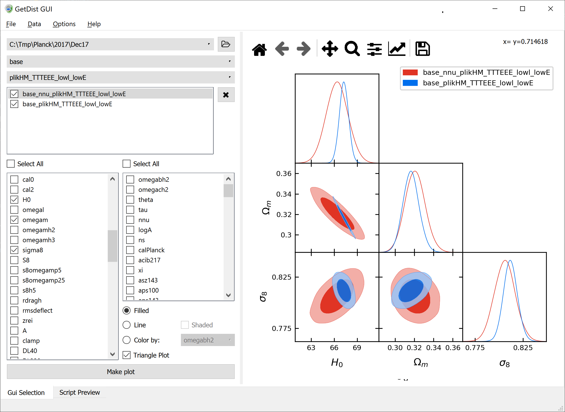
It can open chain files under a selected directory structure (and also [paramgrid](https://cosmologist.info/cosmomc/readme_grids.html) directories as show above,
or [Cobaya grids](https://cobaya.readthedocs.io/en/latest/grids.html)).
See the [intro](https://getdist.readthedocs.io/en/latest/intro.html) for a description of chain file formats. A grid of sample chains files can be
downloaded [here](https://pla.esac.esa.int/pla/#cosmology), after downloading a file just unzip and open the main directory in the GUI.
After opening a directory, you can select each chain root name you want to plot. It is then added to the list box below.
The selected chains can be dragged and dropped to change the order if needed. Then select the parameter names to plot in the checkboxes below that,
and correspond to the names available in the first selected chain.
The Gui supports 1D, 2D (line and filled), 3D (select two parameters and “color by”), and triangle and rectangle plots.
### Script preview
Use the option on the File menu to export a plot as-is to PDF or other image file. For better quality (i.e. not formatted for the current window shape)
and fine control (e.g. add custom legend text, etc), export the script, edit and then run it separately.
The Script Preview tab also gives a convenient way to view the script for the current plot,
and preview exactly what it will produce when run:
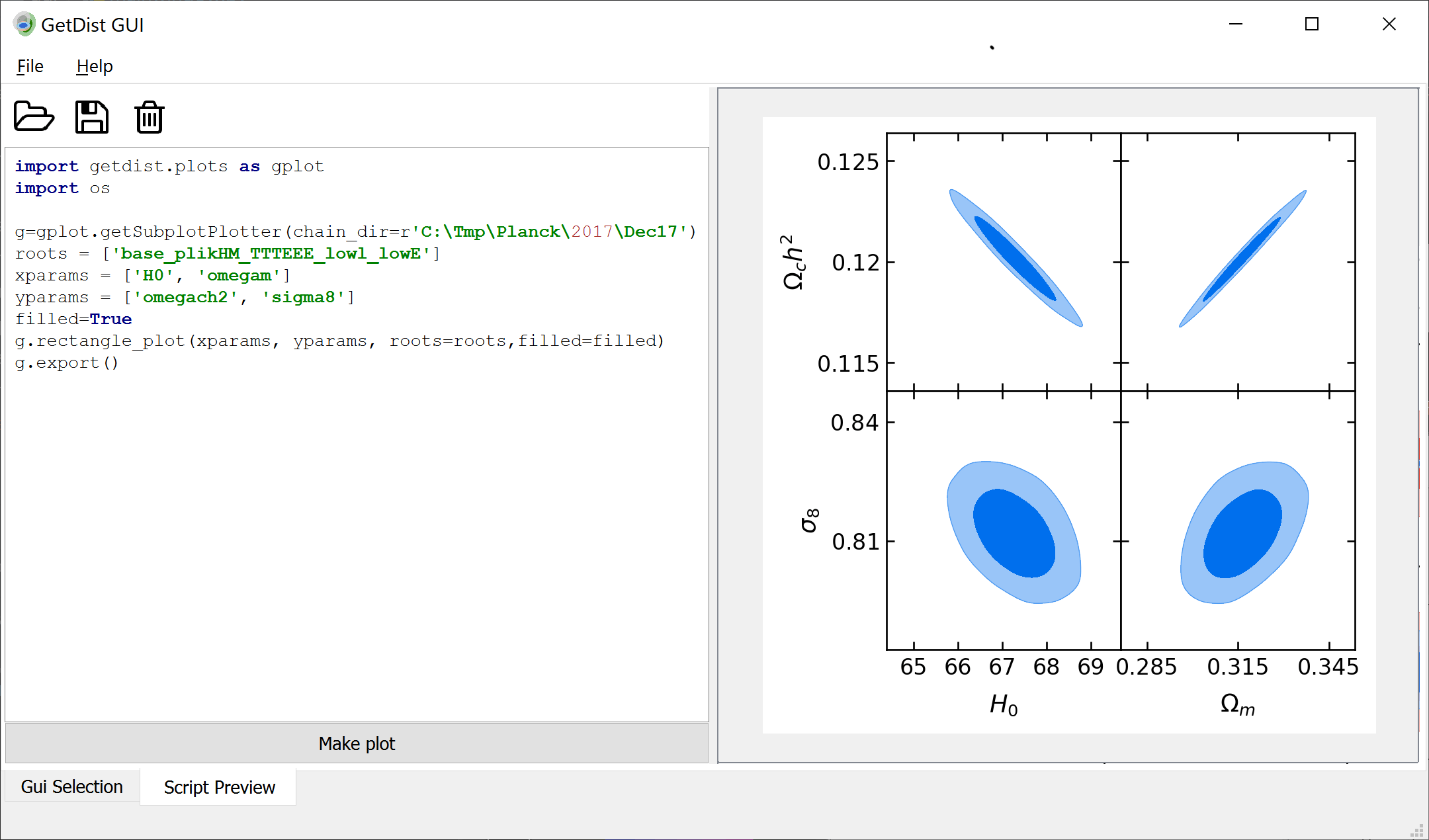
You can also edit and customize the script, or open and play with existing plot scripts.
### Statistics and tables
The Data menu has an option to let you view the parameter statistics (.margestats) and latex tables, convergence stats, and view PCA constraints for
selected parameters. Note that you need a working latex installation to view rendered parameter tables.
### Settings
The Options menu allows you to change a settings defining how limits, lines and contours are calculated, and customize plot options.
The “Plot module config” option lets you use a different module to define the plotting functions (the default is getdist.plots).
#### GUI Script
From python, Run the *getdist-gui* script to run the traditional graphical user interface. This requires [PySide](https://wiki.qt.io/Qt_for_Python) to be installed, but will run on Windows, Linux and Mac.
PySide is not included in default dependencies, but can easily be installed:
```default
pip install PySide6
```
If you have conflicts, with Anaconda/miniconda you can make a consistent new environment
from conda-forge (which includes PySide6), e.g.
```default
conda create -n myenv -c conda-forge scipy matplotlib PyYAML PySide6
```
Once PySide is set up, (re)install getdist and you should then be able to use the getdist-gui script on your path.
NOTE: currently the mac version may crash run this way, use the pre-built installers linked above if you have issues.
### Streamlit-based Web Interface
GetDist also provides a modern web-based interface built with [Streamlit](https://streamlit.io/).
This alternative GUI offers similar functionality to the application but runs in your web browser.
#### Running Locally
To run the Streamlit app locally, you need to install Streamlit first:
```default
pip install streamlit
```
Then you can run the app using the *getdist-streamlit* script. You can also run it directly using
> streamlit run getdist/gui/streamlit_app.py
You can also specify a default directory to open:
```default
getdist-streamlit --dir=/path/to/chains
```
Otherwise the app will automatically look for a default_chains directory in the repository root when it starts.
#### Online Demo
You can try the Streamlit app online at [https://getdist-gui-test.streamlit.app/](https://getdist-gui-test.streamlit.app/).
Note that the online demo:
* Contains fixed example chains (from [https://github.com/cmbant/streamlit-test](https://github.com/cmbant/streamlit-test))
* Cannot upload your own chains (as it’s a demonstration of distributing chains with the app)
* May not work well with very large chains due to limitations of the free Streamlit hosting
#### Features
The Streamlit app includes all the core functionality of the Qt-based GUI, but is not quite as well tested:
* Opening chain directories and grid structures
* Selecting parameters and creating various plot types (1D, 2D, triangle, etc.)
* Viewing statistics and parameter tables
* Customizing analysis settings and plot options
* Exporting plots and scripts
## https://getdist.readthedocs.io/en/latest/intro.html
# GetDist
* **GetDist:**
MCMC sample analysis, plotting and GUI
* **Author:**
Antony Lewis
* **Homepage:**
[https://getdist.readthedocs.io](https://getdist.readthedocs.io)
* **Source:**
[https://github.com/cmbant/getdist](https://github.com/cmbant/getdist)
* **Reference:**
[https://arxiv.org/abs/1910.13970](https://arxiv.org/abs/1910.13970)
[](https://github.com/cmbant/getdist/actions/workflows/tests.yml)[](https://pypi.python.org/pypi/GetDist/)[](https://getdist.readthedocs.io/en/latest)[](https://mybinder.org/v2/gh/cmbant/getdist/master?filepath=docs%2Fplot_gallery.ipynb)[](https://arxiv.org/abs/1910.13970)
## Description
GetDist is a Python package for analysing Monte Carlo samples, including correlated samples
from Markov Chain Monte Carlo (MCMC).
* **Point and click GUI** - select chain files, view plots, marginalized constraints, LaTeX tables and more (Qt-based desktop app and Streamlit web interface)
* **Plotting library** - make custom publication-ready 1D, 2D, 3D-scatter, triangle and other plots
* **Named parameters** - simple handling of many parameters using parameter names, including LaTeX labels and prior bounds
* **Optimized Kernel Density Estimation** - automated optimal bandwidth choice for 1D and 2D densities (Botev et al. Improved Sheather-Jones method), with boundary and bias correction
* **Convergence diagnostics** - including correlation length and diagonalized Gelman-Rubin statistics
* **LaTeX tables** for marginalized 1D constraints
See the [Plot Gallery and tutorial](https://getdist.readthedocs.io/en/latest/plot_gallery.html)
([run online](https://mybinder.org/v2/gh/cmbant/getdist/master?filepath=docs%2Fplot_gallery.ipynb))
and [GetDist Documentation](https://getdist.readthedocs.io/en/latest/index.html).
## Getting Started
Install getdist using pip:
```default
$ pip install getdist
```
or from source files using:
```default
$ pip install -e /path/to/source/
```
You can test if things are working using the unit test by running:
```default
$ python -m unittest getdist.tests.getdist_test
```
Check the dependencies listed in the next section are installed. You can then use the getdist module from your scripts, or
use the GetDist GUI (*getdist-gui* command).
Once installed, the best way to get up to speed is probably to read through
the [Plot Gallery and tutorial](https://getdist.readthedocs.io/en/latest/plot_gallery.html).
## Dependencies
* Python 3.10+
* matplotlib
* scipy
* PySide6 - optional, only needed for Qt-based GUI
* Streamlit - optional, only needed for web-based GUI
* Working LaTeX installation (not essential, only for some plotting/table functions)
Python distributions like Anaconda have most of what you need (except for LaTeX).
To use the Qt-based [GUI](https://getdist.readthedocs.io/en/latest/gui.html) you need PySide6.
To use the Streamlit web interface, you need Streamlit.
See the [GUI docs](https://getdist.readthedocs.io/en/latest/gui.html#installation) for suggestions on how to install both.
## Algorithm details
Details of kernel density estimation (KDE) algorithms and references are give in the GetDist notes
[arXiv:1910.13970](https://arxiv.org/pdf/1910.13970).
## Samples file format
GetDist can be used in scripts and interactively with standard numpy arrays
(as in the [examples](https://getdist.readthedocs.io/en/latest/plot_gallery.html)).
Scripts and the [GetDist GUI](https://getdist.readthedocs.io/en/latest/gui.html) can also read parameter sample/chain files in plain text format
(or in the format output by the [Cobaya](https://cobaya.readthedocs.io) sampling program.
Plain text sample files are of the form:
```default
xxx_1.txt
xxx_2.txt
...
xxx.paramnames
xxx.ranges
```
where “xxx” is some root file name.
The .txt files are separate chain files (there can also be just one xxx.txt file). Each row of each sample .txt file is in the format
> *weight like param1 param2 param3* …
The *weight* gives the number of samples (or importance weight) with these parameters. *like* gives -log(posterior), and *param1, param2…* are the values of the parameters at the sample point. The first two columns can be 1 and 0 if they are not known or used.
The .paramnames file lists the names of the parameters, one per line, optionally followed by a LaTeX label. Names cannot include spaces, and if they end in “\*” they are interpreted as derived (rather than MCMC) parameters, e.g.:
```default
x1 x_1
y1 y_1
x2 x_2
xy* x_1+y_1
```
The .ranges file gives hard bounds for the parameters, e.g.:
```default
x1 -5 5
x2 0 N
```
Note that not all parameters need to be specified, and “N” can be used to denote that a particular upper or lower limit is unbounded. The ranges are used to determine densities and plot bounds if there are samples near the boundary; if there are no samples anywhere near the boundary the ranges have no affect on plot bounds, which are chosen appropriately for the range of the samples.
There can also optionally be a .properties.ini file, which can specify *burn_removed=T* to ensure no burn in is removed, or *ignore_rows=x* to ignore the first
fraction *x* of the file rows (or if *x > 1*, the specified number of rows).
## Loading samples
To load an MCSamples object from text files do:
```default
from getdist import loadMCSamples
samples = loadMCSamples('/path/to/xxx', settings={'ignore_rows':0.3})
```
Here *settings* gives optional parameter settings for the analysis. *ignore_rows* is useful for MCMC chains where you want to
discard some fraction from the start of each chain as burn in (use a number >1 to discard a fixed number of sample lines rather than a fraction).
The MCSamples object can be passed to plot functions, or used to get many results. For example, to plot marginalized parameter densities
for parameter names *x1* and *x2*:
```default
from getdist import plots
g = plots.get_single_plotter()
g.plot_2d(samples, ['x1', 'x2'])
```
When you have many different chain files in the same directory,
plotting can work directly with the root file names. For example to compare *x* and *y* constraints
from two chains with root names *xxx* and *yyy*:
```default
from getdist import plots
g = plots.get_single_plotter(chain_dir='/path/to/', analysis_settings={'ignore_rows':0.3})
g.plot_2d(['xxx','yyy'], ['x', 'y'])
```
MCSamples objects can also be constructed directly from numpy arrays in memory, see the example
in the [Plot Gallery](https://getdist.readthedocs.io/en/latest/plot_gallery.html),
and from, [ArviZ, PyMC and other sampler formats](https://getdist.readthedocs.io/en/latest/arviz_integration.html).
## GetDist script
If you have chain files on on disk, you can also quickly calculate convergence and marginalized statistics using the *getdist* script:
> usage: getdist [-h] [–ignore_rows IGNORE_ROWS] [-V] [ini_file] [chain_root]
> GetDist sample analyser
> positional arguments:
> : *ini_file* .ini file with analysis settings (optional, if omitted uses defaults
>
> *chain_root* Root name of chain to analyse (e.g. chains/test), required unless file_root specified in ini_file
> optional arguments:
where *ini_file* is optionally a .ini file listing *key=value* parameter option values, and chain_root is the root file name of the chains.
For example:
```default
getdist distparams.ini chains/test_chain
```
This produces a set of files containing parameter means and limits (.margestats), N-D likelihood contour boundaries and best-fit sample (.likestats),
convergence diagnostics (.converge), parameter covariance and correlation (.covmat and .corr), and optionally various simple plotting scripts.
If no *ini_file* is given, default settings are used. The *ignore_rows* option allows some of the start of each chain file to be removed as burn in.
To customize settings you can run:
```default
getdist --make_param_file distparams.ini
```
to produce the setting file distparams.ini, edit it, then run with your custom settings.
## GetDist GUI
GetDist provides two graphical user interfaces:
1. **Qt-based Desktop App**: Run *getdist-gui* to use the traditional desktop interface. This requires PySide6 to be installed.
2. **Streamlit Web Interface**: Run *getdist-streamlit* to use the browser-based interface. This requires Streamlit to be installed.
Both interfaces allow you to open a folder of chain files, then easily select, open, plot and compare, as well as viewing standard GetDist outputs and tables.
You can also try the Streamlit interface online at [https://getdist-gui-test.streamlit.app/](https://getdist-gui-test.streamlit.app/) (with fixed example chains).
See the [GUI Documentation](https://getdist.readthedocs.io/en/latest/gui.html) for more details on both interfaces.
## Using with CosmoMC and Cobaya
This GetDist package is general, but is mainly developed for analysing chains from the [CosmoMC](https://cosmologist.info/cosmomc)
and [Cobaya](https://cobaya.readthedocs.io/) sampling programs.
No need to install this package separately if you have a full CosmoMC installation; the Cobaya installation will also install GetDist as a dependency.
Detailed help is available for plotting Planck chains
and using CosmoMC parameter grids in the [Readme](https://cosmologist.info/cosmomc/readme_python.html).
## Citation
You can refer to the JCAP paper:
```default
@article{Lewis:2019xzd,
author = "Lewis, Antony",
title = "{GetDist: a Python package for analysing Monte Carlo samples}",
eprint = "1910.13970",
archivePrefix = "arXiv",
primaryClass = "astro-ph.IM",
doi = "10.1088/1475-7516/2025/08/025",
journal = "JCAP",
volume = "08",
pages = "025",
year = "2025"
}
```
and references therein as appropriate.
## LLM Integration
For AI assistants and LLM agents working with GetDist, a single-file context document is available at [GetDist LLM Context](https://help.cosmologist.info/api/context/getdist). This document provides a comprehensive overview of GetDist’s functionality, common usage patterns, and best practices in a format optimized for LLM context windows.
## Contributing
Please see the [Contributing Guide](https://github.com/cmbant/getdist/blob/master/CONTRIBUTING.md).
---
[](https://www.sussex.ac.uk/astronomy/)[](https://erc.europa.eu/)[](https://stfc.ukri.org/)
## Usage examples from plot_gallery jupyter notebook
GetDist Jupyter Notebook Plot Gallery
===============
Demonstrates the types of plot you can make with [GetDist](https://getdist.readthedocs.io) and how to make them.
You can also [run this notebook online](https://mybinder.org/v2/gh/cmbant/getdist/master?filepath=docs%2Fplot_gallery.ipynb).
```python
# Show plots inline, and load main getdist plot module and samples class
%matplotlib inline
%config InlineBackend.figure_format = 'retina'
import os
import sys
sys.path.insert(0, os.path.realpath(os.path.join(os.getcwd(), "..")))
import getdist
import IPython
import matplotlib
import matplotlib.pyplot as plt
from getdist import MCSamples, plots
print("GetDist Version: %s, Matplotlib version: %s" % (getdist.__version__, matplotlib.__version__))
```
```python
# use this here *after* the above (instead of matplotlib inline) to use interactive plots
# %matplotlib notebook
```
```python
# Get some random samples for demonstration:
# make random covariance, then independent samples from Gaussian
import numpy as np
ndim = 4
nsamp = 10000
random_state = np.random.default_rng(10) # seed random generator
A = random_state.random((ndim, ndim))
cov = np.dot(A, A.T)
samps = random_state.multivariate_normal([0] * ndim, cov, size=nsamp)
A = random_state.random((ndim, ndim))
cov = np.dot(A, A.T)
samps2 = random_state.multivariate_normal([0] * ndim, cov, size=nsamp)
```
```python
# Get the getdist MCSamples objects for the samples, specifying same parameter
# names and labels; if not specified weights are assumed to all be unity
names = ["x%s" % i for i in range(ndim)]
labels = ["x_%s" % i for i in range(ndim)]
samples = MCSamples(samples=samps, names=names, labels=labels)
samples2 = MCSamples(samples=samps2, names=names, labels=labels, label="Second set")
```
```python
# Triangle plot (sometimes also called a corner plot)
g = plots.get_subplot_plotter()
g.triangle_plot([samples, samples2], filled=True)
```
```python
# Here we are using inline plots, but if you wanted to export to file you'd just do e.g.
# g.export('output_file.pdf')
```
```python
# 1D marginalized plot
g = plots.get_single_plotter(width_inch=4)
g.plot_1d(samples, "x2")
```
```python
# 1D marginalized comparison plot
g = plots.get_single_plotter(width_inch=3)
g.plot_1d([samples, samples2], "x1")
```
```python
# 1D normalized comparison plot
g = plots.get_single_plotter(width_inch=4)
g.plot_1d([samples, samples2], "x1", normalized=True)
```
```python
# 2D line contour comparison plot with extra bands and markers
g = plots.get_single_plotter()
g.plot_2d([samples, samples2], "x1", "x2")
g.add_x_marker(0)
g.add_y_bands(0, 1)
```
```python
# Filled 2D comparison plot with legend
g = plots.get_single_plotter(width_inch=4, ratio=1)
g.plot_2d([samples, samples2], "x1", "x2", filled=True)
g.add_legend(["sim 1", "sim 2"], colored_text=True);
```
```python
# Shaded 2D comparison plot
g = plots.get_single_plotter(width_inch=4)
g.plot_2d([samples, samples2], "x1", "x2", shaded=True);
```
```python
# Customized 2D filled comparison plot
g = plots.get_single_plotter(width_inch=6, ratio=3 / 5.0)
g.settings.legend_fontsize = 12
g.plot_2d([samples, samples2], "x1", "x2", filled=True, colors=["green", ("#F7BAA6", "#E03424")], lims=[-4, 7, -5, 5])
g.add_legend(["Sim ", "Sim 2"], legend_loc="upper right");
```
```python
# Change the contours levels for marge stats and plots
# (note you need a lot of samples for 99% confidence contours to be accurate)
g = plots.get_single_plotter()
samples.updateSettings({"contours": [0.68, 0.95, 0.99]})
g.settings.num_plot_contours = 3
g.plot_2d(samples, "x1", "x2");
```
```python
# 2D scatter (3D) plot
g = plots.get_single_plotter(width_inch=5)
g.plot_3d(samples, ["x1", "x2", "x3"])
```
```python
# Multiple 1D subplots
g = plots.get_subplot_plotter(width_inch=5)
g.plots_1d(samples, ["x0", "x1", "x2", "x3"], nx=2);
```
```python
# Multiple 2D subplots
g = plots.get_subplot_plotter(subplot_size=2.5)
g.settings.scaling = False # prevent scaling down font sizes even though small subplots
g.plots_2d(samples, param_pairs=[["x0", "x1"], ["x2", "x3"]], nx=2, filled=True);
```
```python
# Customized triangle plot
g = plots.get_subplot_plotter()
g.settings.figure_legend_frame = False
g.settings.alpha_filled_add = 0.4
g.settings.title_limit_fontsize = 14
g.triangle_plot(
[samples, samples2],
["x0", "x1", "x2"],
filled=True,
legend_labels=["Simulation", "Simulation 2"],
legend_loc="upper right",
line_args=[{"ls": "--", "color": "green"}, {"lw": 2, "color": "darkblue"}],
contour_colors=["green", "darkblue"],
title_limit=1, # first title limit (for 1D plots) is 68% by default
markers={"x2": 0},
marker_args={"lw": 1},
)
```
---
If you prefer to use one of the standard color series you can do that, using the matplotlib [named colormaps](https://matplotlib.org/examples/color/colormaps_reference.html)
```python
# tab10 is the standard discrete color table (good for color blindness etc.)
g = plots.get_subplot_plotter(subplot_size=2)
# Set line style default
g.settings.line_styles = "tab10"
g.plots_1d([samples, samples2], ["x1", "x2", "x3"], nx=3, legend_ncol=2, lws=[3, 2])
# or set explicitly
g.plots_1d([samples, samples2], ["x1", "x2", "x3"], nx=3, legend_ncol=2, colors="Set1", ls=["-", "--"])
# For filled contours set solid_colors setting (or set contour_colors argument as above)
g.settings.solid_colors = "tab10"
g.triangle_plot([samples, samples2], ["x1", "x2"], filled=True, contour_lws=2)
```
```python
# 3D (scatter) triangle plot
g = plots.get_subplot_plotter(width_inch=6)
# you can adjust the scaling factor if font sizes are too small when
# making many subplots in a fixed size (default=2 would give smaller fonts)
g.settings.scaling_factor = 1
g.triangle_plot(
[samples, samples2], ["x1", "x2", "x3"], plot_3d_with_param="x0", legend_labels=["Simulation", "Simulation 2"]
)
```
```python
# You can reference g.subplots for manual tweaking,
# e.g. let's add a vertical axis line in the first column
# (this can also be done directly via the markers argument to triangle_plot)
for ax in g.subplots[:, 0]:
ax.axvline(0, color="gray", ls="--")
IPython.display.display(g.fig)
```
```python
# Rectangle 2D comparison plots
g = plots.get_subplot_plotter()
g.settings.figure_legend_frame = False
g.rectangle_plot(
["x0", "x1"],
["x2", "x3"],
roots=[samples, samples2],
filled=True,
plot_texts=[["Test Label", None], ["Test 2", None]],
);
```
```python
# Or join rows of 1D or 2D plots.
from matplotlib import cm
g.settings.linewidth = 2
g.plots_1d([samples, samples2], share_y=True, nx=2, legend_ncol=2, colors=cm.tab10)
g.rectangle_plot(["x1", "x2", "x3"], "x0", roots=[samples, samples2], colors=["k", "C2"]);
```
```python
# Example of how to handle boundaries (samples are restricted to x0 >-0.5)
cut_samps = samps[samps[:, 0] > -0.5, :]
cut_samples = MCSamples(samples=cut_samps, names=names, labels=labels, ranges={"x0": (-0.5, None)}, label="Cut samples")
g = plots.get_subplot_plotter(subplot_size=2)
g.settings.title_limit_fontsize = 14 # reference size for 3.5 inch subplot
g.plots_1d(cut_samples, nx=4, title_limit=2) # title by 95% limit
g = plots.get_single_plotter(width_inch=4, ratio=1)
g.plot_2d(cut_samples, "x0", "x1", filled=True);
```
```python
# Periodic parameter: for samples within a perioidic range, you can also specify that by use a 3-tuple for the range
# This ensures the densities at the two sides agree, and reduces sampling noise near the boundaries
# (but is not fully optimized for bandwidth selection)
def func(x): # perioid function
return 0.8 * np.sin(x + 0.5) ** 2 + 0.2
rng = np.random.default_rng(10)
sample_array = rng.uniform(0, np.pi, 12500)
r = rng.uniform(0, 1, len(sample_array))
p = []
for x, rand in zip(sample_array, r):
if rand < func(x):
p.append(x)
samps = MCSamples(samples=np.array(p), names=["x"], ranges={"x": [0, np.pi]})
samps2 = MCSamples(samples=np.array(p), names=["x"], ranges={"x": [0, np.pi, True]})
gplot = plots.get_single_plotter(width_inch=4)
gplot.plot_1d(samps, "x")
gplot.plot_1d(samps2, "x", colors=["r"])
x = np.arange(0, np.pi, 0.01)
plt.plot(x, func(x), ls="--")
plt.xlim(0, np.pi)
plt.ylim(0, None)
plt.legend(["Non-periodic", "Periodic", "True distribution"]);
```
```python
# Add and plot a new derived parameter
# getParms gets p so that p.x0, p.x1.. are numpy vectors of sample values
# For individual parameters you can also just do samples['x0'] etc.
p = samples.getParams()
assert np.all(p.x1 == samples["x1"])
samples.addDerived((5 + p.x2) ** 2, name="z", label="z_d")
g = plots.get_subplot_plotter(subplot_size=4)
g.plots_2d(samples, "x1", ["x2", "z"], nx=2);
```
```python
# Example of how to do importance sampling, modifying the samples by re-weighting by a new likelihood
# e.g. to modify samples to be from the original distribution times a Gaussian in x1
# (centered on 1, with sigma=1.2)
# Using samples['x'] retrieves the vector of sample values for the parameter named 'x'
new_samples = samples.copy() # make a copy so don't change the original
new_loglike = (samples["x1"] - 1) ** 2 / 1.2**2 / 2
# code currently assumes existing loglikes are set, set to zero here
new_samples.loglikes = np.zeros(samples.numrows)
# re-weight to account for the new likelihood
new_samples.reweightAddingLogLikes(new_loglike)
g = plots.get_single_plotter(width_inch=4, ratio=1)
g.plot_2d([samples, new_samples], "x0", "x1", filled=True);
```
```python
# You can also account for general 2D prior boundary cuts that are not aligned with the axes
# (Note that the auto-smoothing kernel size does not account for non-trivial mask
# so may want to manually adjust the kernel smoothing width [smooth_scale_2D])
# e.g. consider cut that is linear function of two parameters with these parameters
y0 = -0.7
x0 = -0.2
r = 0.3
def mask_function(minx, miny, stepx, stepy, mask):
# define function to tell getdist which 2D points are excluded by the prior
# Note this should not include min, max parameter range cuts aligned with axes, which are handled as above.
x = np.arange(mask.shape[1]) * stepx + minx
y = np.arange(mask.shape[0]) * stepy + miny
# Create 2D coordinate grids
X, Y = np.meshgrid(x, y)
# Zero out the array where prior excluded
mask[Y < y0 - r * (X - x0)] = 0
cut_samps = samples.copy()
p = cut_samps.getParams()
cut_samps.filter(p.x1 - y0 + (p.x0 - x0) * r > 0) # make test samples with hard prior cut
g = plots.get_single_plotter(width_inch=4, ratio=0.9)
# mass in the mask function so getdist knows about the prior cut
g.plot_2d(cut_samps, "x0", "x1", filled=True, mask_function=mask_function)
g.add_2d_contours(cut_samps, "x0", "x1", filled=False, color="g", ls="--")
x = np.linspace(-5, 5, 100)
plt.plot(x, y0 - r * (x - x0), color="k", ls="--")
g.add_legend(["prior mask corrected", "uncorrected"])
g.export("z:\\boundaries2D.pdf")
```
```python
# Many other things you can do besides plot, e.g. get latex
# Default limits are 1: 68%, 2: 95%, 3: 99% probability enclosed
# See https://getdist.readthedocs.io/en/latest/analysis_settings.html
# and examples for below for changing analysis settings
# (e.g. 2hidh limits, and how they are defined)
print(cut_samples.getInlineLatex("x0", limit=2))
print(samples.getInlineLatex("x0", limit=2))
```
```python
print(samples.getInlineLatex("x1", limit=1))
```
```python
print(samples.getTable().tableTex())
```
```python
# results from multiple chains
from getdist.types import ResultTable
print(
ResultTable(
ncol=1, results=[samples, new_samples], paramList=["x0", "x3"], limit=1, titles=["Samples", "Weighted samples"]
).tableTex()
)
```
```python
print(samples.PCA(["x1", "x2"]))
```
```python
stats = cut_samples.getMargeStats()
lims0 = stats.parWithName("x0").limits
lims1 = stats.parWithName("x1").limits
for conf, lim0, lim1 in zip(samples.contours, lims0, lims1):
print("x0 %s%% lower: %.3f upper: %.3f (%s)" % (conf, lim0.lower, lim0.upper, lim0.limitType()))
print("x1 %s%% lower: %.3f upper: %.3f (%s)" % (conf, lim1.lower, lim1.upper, lim1.limitType()))
```
```python
# if samples have likelihood values, can also get best fit sample and extremal values of N-D confidence region
# Note in high dimensions best-fit sample is likely a long way from the best fit; N-D limits also often MC-noisy
print(new_samples.getLikeStats())
print(
"x0 95% n-D confidence extrema:",
new_samples.paramNames.parWithName("x0").ND_limit_bot[1],
new_samples.paramNames.parWithName("x0").ND_limit_top[1],
)
```
```python
# Save to file
import os
import tempfile
tempdir = os.path.join(tempfile.gettempdir(), "testchaindir")
if not os.path.exists(tempdir):
os.makedirs(tempdir)
rootname = os.path.join(tempdir, "testchain")
samples.saveAsText(rootname)
```
```python
# Load from file
from getdist import loadMCSamples
readsamps = loadMCSamples(rootname)
```
```python
# Make plots from chain files, loading automatically as needed by using root file name
g = plots.get_single_plotter(chain_dir=tempdir, width_inch=4)
g.plot_2d("testchain", "x1", "x2", shaded=True);
```
```python
# Custom settings for all loaded chains can be set as follows;
# for example to use custom contours and remove the first 20% of each chain as burn in
g = plots.get_single_plotter(
chain_dir=tempdir, analysis_settings={"ignore_rows": 0.2, "contours": [0.2, 0.4, 0.6, 0.8]}
)
g.settings.num_plot_contours = 4
g.plot_2d("testchain", "x1", "x2", filled=False);
```
```python
# Silence messages about load
getdist.chains.print_load_details = False
```
```python
# Chains can be loaded by searching in multiple directories by giving a list as chain_dir
# (note chain names must be unique)
# make second test chain in new temp dir
temp2 = os.path.join(tempdir, "chaindir2")
cut_samples.saveAsText(os.path.join(temp2, "testchain2"), make_dirs=True)
# Plot from chain files
g = plots.get_single_plotter(chain_dir=[tempdir, temp2])
g.plot_2d(["testchain", "testchain2"], "x1", "x2", filled=True);
```
```python
# You can also load a samples object from the chain directories for further manipulation
read_samples = g.samples_for_root("testchain")
# e.g. add a new derived parameter
# Note our new variable is >0 by definition, so also need to define its finite range to
# get correct densities near zero
p = read_samples.getParams()
read_samples.addDerived(np.abs(p.x1), name="modx1", label="|x_1|", range=[0, None])
g.new_plot()
g.plot_2d(read_samples, "modx1", "x2", filled=True);
```
```python
# cleanup test files
import shutil
shutil.rmtree(tempdir)
```
```python
# The plotting scripts also let you plot Gaussian (or Gaussian mixture) contours
# This is useful for plotting smooth theory results, e.g. Fisher forecasts.
from getdist.gaussian_mixtures import GaussianND
covariance = [[0.001**2, 0.0006 * 0.05, 0], [0.0006 * 0.05, 0.05**2, 0.2**2], [0, 0.2**2, 2**2]]
mean = [0.02, 1, -2]
gauss = GaussianND(mean, covariance)
g = plots.get_subplot_plotter()
g.triangle_plot(gauss, filled=True)
```
```python
# You can also explicitly name parameters so Gaussian mixtures can be plotted
# in combination with samples
from getdist.gaussian_mixtures import Mixture2D
cov1 = [[0.001**2, 0.0006 * 0.05], [0.0006 * 0.05, 0.05**2]]
cov2 = [[0.001**2, -0.0006 * 0.05], [-0.0006 * 0.05, 0.05**2]]
mean1 = [0.02, 0.2]
mean2 = [0.023, 0.09]
mixture = Mixture2D([mean1, mean2], [cov1, cov2], names=["zobs", "t"], labels=[r"z_{\rm obs}", "t"], label="Model")
# Generate samples from the mixture as simple example
mix_samples = mixture.MCSamples(3000, label="Samples")
g = plots.get_subplot_plotter()
# compare the analytic mixture to the sample density
g.triangle_plot([mix_samples, mixture], filled=False)
```
```python
# For long tick labels GetDist will space them intelligently so they don't overlap.
# You can also rotate tick labels
p = mix_samples.getParams()
mix_samples.addDerived(10 * p.zobs - p.t / 10, name="xt", label="x_t")
g = plots.get_subplot_plotter(subplot_size=3)
g.settings.axes_fontsize = 12
g.settings.axis_tick_x_rotation = 45
g.settings.axis_tick_y_rotation = 90
g.settings.colorbar_tick_rotation = 90
g.triangle_plot(mix_samples, ["t", "zobs"], plot_3d_with_param="xt", filled=True)
```
```python
# Double triangle plot
g = plots.get_subplot_plotter()
g.triangle_plot(
[samples, new_samples],
["x0", "x1", "x2"],
filled=True,
upper_roots=[samples2],
upper_kwargs={"contour_colors": ["green"]},
legend_labels=["Samples", "Reweighted samples", "Second samples"],
);
```
```python
# Variants
from matplotlib import cm
g = plots.get_subplot_plotter()
upper_kwargs = {
"contour_colors": cm.tab10.colors[4:],
"contour_ls": ["-", "--"],
"filled": [True, False],
"show_1d": [True, True],
"contour_lws": [1, 2],
}
g.settings.solid_contour_palefactor = 0.9
g.settings.alpha_filled_add = 0.6
g.triangle_plot(
[samples, new_samples],
["x0", "x1", "x2"],
filled=True,
contour_colors=["C3", "green"],
markers={"x0": -0.5},
upper_roots=[samples2, cut_samples],
upper_kwargs=upper_kwargs,
upper_label_right=True,
legend_labels=["Samples", "Reweighted", "Second", "Cut"],
);
```
```python
# Sets of 3D plots
g = plots.get_subplot_plotter(width_inch=8)
g.plots_3d(mix_samples, [["xt", "t", "zobs"], ["t", "zobs", "xt"]], nx=2)
# and this is how to manually add contours only to a specific plot
g.add_2d_contours(mixture, "t", "zobs", ax=[0, 1]);
```
```python
# 4D x-y-z-color scatter plots:
# Use ""%matplotlib notebook" to interactively rotate etc.
g = plots.get_single_plotter()
g.plot_4d(
[samples, samples2],
["x0", "x1", "x2", "x3"],
cmap="viridis",
color_bar=False,
azim=75,
alpha=[0.3, 0.1],
shadow_color=False,
compare_colors=["k"],
)
```
```python
# with projection onto axes, colorbar, custom limits, colors, etc.
g = plots.get_single_plotter()
g.plot_4d(
samples,
["x0", "x1", "x2", "x3"],
cmap="jet",
alpha=0.4,
shadow_alpha=0.05,
shadow_color=True,
max_scatter_points=6000,
lims={"x2": (-3, 3), "x3": (-3, 3)},
colorbar_args={"shrink": 0.6},
)
```
```python
# use animate=True and mp4_filename option to export an rotation animation
# this shows example output
from IPython.display import Video
Video("https://cdn.cosmologist.info/antony/sample_rotation.mp4", html_attributes="controls loop", width=600)
```
---
**Using styles to change settings for consistent plot scripts**
If you want to change several default settings, you can make a module containing a new
plotter class, which defines its own settings and behaviour, and then use it as a style.
A couple of sample styles are included: getdist.styles.tab10 and getdist.styles.planck.
Using the same style in each script will then give consistent outputs without changing settings
each time.
```python
# use the 'tab10' style, which uses default matplotlib colourmaps
from getdist.styles.tab10 import style_name
plots.set_active_style(style_name)
g = plots.get_subplot_plotter(width_inch=6)
g.triangle_plot(
[samples, samples2], ["x1", "x2", "x3"], plot_3d_with_param="x0", legend_labels=["Simulation", "Simulation 2"]
)
```
```python
# getdist.styles.planck is a more complicated case which also changes matplotlib style
# (to use latex rendering and different fonts). It also turns of scaling by default so all
# fonts are fixed size.
from getdist.styles.planck import style_name
plots.set_active_style(style_name)
g = plots.get_subplot_plotter(width_inch=6)
g.triangle_plot(
[samples, samples2], ["x1", "x2", "x3"], plot_3d_with_param="x0", legend_labels=["Simulation", "Simulation 2"]
)
```
```python
# Back to default style
plots.set_active_style();
```
**Getting consistent sizes for publication**
By default, font and line sizes are scaled for small plots, which is often necessary if making
figures with many subplots in. Setting parameters like settings.fontsizes, settings.axes_labelsize are specified at a reference axis size (defaul 3.5 inches); for smaller plots they are reduced.
For publication you may wish to have constent font sizes between figures, and hence specify fixed sizes and use a fixed figure size.
```python
# width_inch=3.5 is often good for a one-column figure.
# If we make one figure or multiple subplots, by deafult font sizes will
# be different for smaller axis sizes
g = plots.get_single_plotter(width_inch=6)
g.plot_2d([samples, cut_samples], ["x1", "x2"])
g.add_legend(["Label 1", "Label 2"], legend_loc="lower right")
# finish_plot will call tight_layout to make sure everything is
# actually within the requested figure size, so plots saved at consistent size
g = plots.get_single_plotter(width_inch=3.5)
g.plot_2d([samples, cut_samples], ["x1", "x2"])
g.add_legend(["Label 1", "Label 2"], legend_loc="lower right")
g.add_text("Text label", 0.1, 0.9)
g = plots.get_subplot_plotter(width_inch=3.5)
g.triangle_plot([samples, cut_samples], ["x1", "x2", "x3"], legend_labels=["Label1", "Label2"])
g.add_text("A", 0.2, 0.8, ax=g.subplots[1, 0], color="blue")
# finish_plot is not needed for commands which generate sets of subplots
```
```python
# The scaling_factor determines how quickly fonts shrink (default 2).
# Using scaling_factor=1 will give somewhat larger font sizes after scaling
g = plots.get_subplot_plotter(width_inch=3.5)
g.settings.scaling_factor = 1.5
g.triangle_plot([samples, cut_samples], ["x1", "x2", "x3"], legend_labels=["Label1", "Label2"])
g.add_text("A", 0.2, 0.8, ax=g.subplots[1, 0], color="blue")
```
```python
# Scaling is entirely disabled by setting settings.scaling=False or
# getting the plotter instance using scaling=False.
# Here font sizes and line widths are all consistent:
g = plots.get_single_plotter(width_inch=3.5, scaling=False)
g.plot_2d([samples, cut_samples], ["x1", "x2"])
g.add_text("Text label", 0.1, 0.9)
g.add_legend(["Label 1", "Label 2"], legend_loc="lower right")
plt.suptitle(
"Default font sizes are tick labels:\n %.2g, labels: %.2g, legend: %.2g, text: %.2g"
% (g.settings.axes_fontsize, g.settings.axes_labelsize, g.settings.legend_fontsize, g.settings.fontsize),
va="bottom",
)
g.triangle_plot([samples, cut_samples], ["x1", "x2", "x3"], legend_labels=["Label1", "Label2"])
g.add_text("A", 0.2, 0.8, ax=g.subplots[1, 0], color="blue")
```
```python
# You can also set default font settings to the values set in your rcParams
g = plots.get_subplot_plotter(width_inch=3.5, scaling=False, rc_sizes=True)
g.triangle_plot([samples, cut_samples], ["x1", "x2", "x3"], legend_labels=["Label1", "Label2"])
g.add_text("A", 0.2, 0.8, ax=("x1", "x2"), color="blue")
plt.suptitle(
"rc font sizes are tick labels:\n %.2g, labels: %.2g, legend: %.2g, fontsize: %.2g"
% (g.settings.axes_fontsize, g.settings.axes_labelsize, g.settings.legend_fontsize, g.settings.fontsize),
va="bottom",
);
```
---
**Controlling analysis settings**
The default kernel density estimation setting usually give good results, but note that contours can seem quite smooth even if the residual sampling noise is quite large. You can change the [analysis settings](https://getdist.readthedocs.io/en/latest/analysis_settings.html) from the default to visually inspect the stability of the result.
```python
ndim = 4
nsamp = 400
A = random_state.random((ndim, ndim))
cov = np.dot(A, A.T)
samps = random_state.multivariate_normal([0] * ndim, cov, size=nsamp)
names = ["x%s" % i for i in range(ndim)]
labels = ["x_%s" % i for i in range(ndim)]
# default settings attempt to minimize sampling noise and bias
s1 = MCSamples(samples=samps, names=names, labels=labels, label="Default")
# Use standard lowest-order kernel density estimates the contours get visually more noisy
# (and more biased). Kernel widths are determined automatically.
s2 = MCSamples(
samples=samps,
names=names,
labels=labels,
label="Lowest-order (Parzen) kernel",
settings={"mult_bias_correction_order": 0},
)
# manually set the smoothing scale in units of the standard deviation
# Can also use copy() to generate a copy of samples with new settings
s3 = s2.copy(
label=r"Lowest-order with $0.3\sigma$ smoothing",
settings={"mult_bias_correction_order": 0, "smooth_scale_2D": 0.3, "smooth_scale_1D": 0.3},
)
g = plots.get_subplot_plotter()
g.triangle_plot([s1, s2, s3], filled=False)
# Note that for some flat distributions the location of 2D equal-enclosed-probability contours can
# be very unstable, e.g. a flat bounded distribution 0 xcut]
plt.figure(figsize=(6, 4))
plt.hist(samps, bins=50)
plt.title("Sample Histogram")
for mult_order in [0, 1]:
# Incorrectly set samples without specifying the prior range
no_range = MCSamples(samples=samps, names=["x"], settings={"mult_bias_correction_order": mult_order})
# For parameters with hard priors you must specify the range, here p>xcut by definition
with_range = MCSamples(
samples=samps, names=["x"], settings={"mult_bias_correction_order": mult_order}, ranges={"x": [xcut, None]}
)
snone = with_range.copy(settings={"boundary_correction_order": -1, "mult_bias_correction_order": mult_order})
s0 = with_range.copy(settings={"boundary_correction_order": 0, "mult_bias_correction_order": mult_order})
g = plots.get_single_plotter(width_inch=6)
g.settings.norm_prob_label = "$P(x)$"
g.plot_1d([no_range, snone, s0, with_range], "x", normalized=True)
# Plot true distribution (normalized to peak 1)
x = np.arange(xcut, 5, 0.01)
dist = np.exp(-(x**2) / 2 + xcut**2 / 2)
dist /= np.sum(dist) * 0.01
g.get_axes().plot(x, dist, ls="--", color="magenta")
g.add_x_marker(xcut, lw=1)
plt.title("Kernel densities, %s multiplicative boundary correction" % ("with" if mult_order else "without"))
g.add_legend(
legend_labels=[
"No range, bad auto-bandwidth",
"No boundary correction",
"0th order boundary correction",
"1st order correction (default)",
"True sampled distribution",
],
legend_loc="upper right",
)
```
***
**Further Reading**
See the full [documentation](https://getdist.readthedocs.io/en/latest/index.html) for further details and examples